Investigat Hydraulic Performance of Groins by Computational Fluid Dynamic Model

International Journal of Scientific & Engineering Research, Volume 5, Issue ŗŘ, ber-2014

ISSN 2229-5518

143

In vest i gat Hyd r au l i c Per f or man ce of Gr oi ns b y Co m pu tat i o nal Fl ui d Dyn ami c

Mod el

Asst. Prof. Dr. Laith Jawad Aziz, Maryam Taha Nasret

Abstracted-Three dimensional Computational Fluid Dynamic (CFD) model are intend to investigate the flow patterns around groins under different conditions. Used k- turbulent model and VOF method to predict the complex flow around groins .The initial part of this study con- cerns to the experimental investigations of flow patterns. The results from the measurements in terms of water elevation, velocity magnitudes according to groins are showed. These were used to validate the Computational Fluid Dynamic model. The results of CFD models showed good agreements with the corresponding experimental measurements.
Many aspects were conducted on the CFD model for most important design parameters, such as, Contraction ratio (Lg/B), and Orientations. Results showed that, the Reattachment length is about 12-13 times the impermeable Groins length; Groins with (Lg/B) more than 20% will increased the velocity and shear stress by 76, and 99 % respectively, Groins oriented either normal to the flow or slightly downstream for best performance. Groins oriented on downstream reduces scour (shear stress) at the end of the groins by 50%.
Index Terms- CFD, Groins, k- turbulent model, Reattachment length, VOF, multiphase flow, mesh independent solutions.
——————————  ——————————

1.INTRODUCTION

roins are structures that protrude into rivers from the bank and a suitable measure for bank protection and flood control, it's also one of the widely used river train-

ing structures due to the well-known characteristics of redi- recting the flow to keep away from erodible banks and pre- serve the desired depth of a river channel for navigation (Carl- ing et al, 1996).
Groins may be built as a single structure, namely a single groin, or as a series of groins built in a row, along with one or both sides of a river as a groin field. Figure (1) shows an exam- ple of a single groin and field of groins, Figures (2), and (3) shows two examples of application of groin fields, and the other case study for the bank failure caused by the absence of the groins on the river bank (Marchland in Louisiana), which oc- curred in 1983.
Recently groins have been received more attention from the
standpoint of ecosystem. The design, location, orientation and
length of groins are very important subjects for the hydraulic
engineers in the field. Basically, it is important to have a clear
picture of flow phenomenon around these structures in order
to be able to make a safe and economic design. Also, hydraulic conditions such as velocity, water depth, bed shape, and bed
material around groins are so diverse to provide the ecosys- tem with suitable habitat. (Shields et al., 1995).
The characteristics of this kind of structure are usually stu- died through laboratory using experimental channels under controlled conditions which are expensive and sometimes cannot reproduce all the situations that one requires to study the flow and sediment transport in rivers which is a matter of considerable interesting in the field of river engineering and sedimentation research (Graf, 1970; Ouillon and Dartus, 1997; Chang and Scotti, 2003; Schulz, 2003; Sekiguchi et al., 2004; Nagata et al., 2005).(quoted from ,Teraguchi, H.,2011)
Despite the research efforts made so far the effects of these structures on the flow conditions and bed morphology changes are not sufficiently known yet, that is why further investigations using up-to-date techniques are necessary.
In order to describe the spatial turbulence complexity of flow accurately around groins, 3D numerical models need to be used. Therefore, in the last decades due to the fast develop- ment of new computational techniques, CFD (Computational Fluid Dynamic) models have progressively become more of a competitor to laboratory experiments.

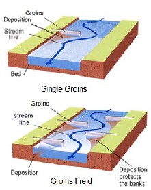
Figure (1) Sketch of groins

International Journal of Scientific & Engineering Research Volume 5, Issue ŗŘǰȱ ȬŘŖŗŚȱȱ

ISSN 2229-5518

144

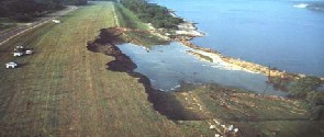
FIGURE (2) APPLICATION OF GROINS FOR IMPROVEMENT OF NAVIGATION,

AND BANK PROTECTION IN RIVERS (TERAGUCHI, 2011)

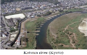
FIGURE (3) ABSENCE OF GROINS MAY CAUSE THE BANK FAILURE, MARCHLAND IN LOUISIANA, WHICH OCCURRED IN 1983.

2. DESCRIPTION OF EXPERIMENTAL SET-UP

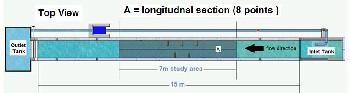
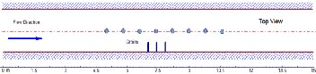
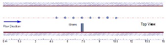
The experiments were carried out in a flume located at the hydraulics Laboratory of, Kufa University- Faculty of Engi- neering- Iraq. Figure (4) below represent the sketch of flume. In the present experiments, this type of groin was made by a wood plate with 1.5 cm thickness, 7.5 cm length perpendicular to flow direction and 30.0 cm height above the initial flat bed level.
One of the primary objectives of these experiments is to exam- ine the effect of variation in the shapes of groins on flow pat- terns. Moreover, the ability of the numerical model to simulate the experimental results is checked comparatively in this chapter and. The following images represent the steps of the experimental test for each scenario as shown in Figure (5).

————————————————

• Asst. Prof. Dr. Laith Jawad aziz, is currently one of staff at faculity of engineering in Universityof kufa. Iraq. E-mail: laithja@eng.kuiraq.com

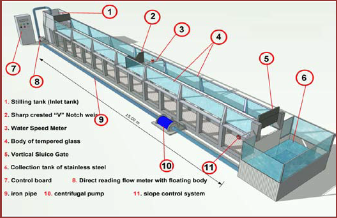
Figure (5) sketch of flume for exprimntal work

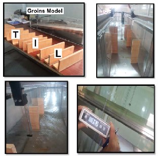
Figure (5) step by step for expremintal work

The recorded data in table (1),(2),and (3) represent the velocity distribution through a selected point along of canal as seen in figures (6) ,(7), and (8) for laboratory case (measured velocity) and theoretical case (CFD velocity).
The results of the CFD model shows a good agreement with the experimental results over a large part of the curve, espe- cially when the points are near from upstream side . Some of points on downstream side have small difference causes by turbulence of outlet of flume.

• Maryam Taha Nasret ,is currently pursuing masters degree program in Civil engineering in University of Kufa , Iraq. E-mail: ma- ryam_nasret@yahoo.com

International Journal of Scientific & Engineering Research Volume 5, Issue ŗŘǰȱ ȬŘŖŗŚȱȱ

ISSN 2229-5518

145

Senario 1: Flume without Groins

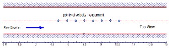
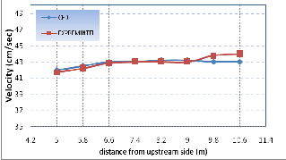
Figure (6) Velocity distribution (measured &CFD) (Scenario

Senario 2: Flume with Single Straight Groin:

The fellowing figures represent the mesuread and CFD veloci- ty for scenario 2

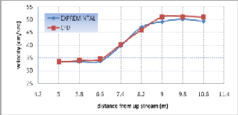
Figure (7) Velocity distribution (measured &CFD) (Scenario 2)

Senario 3: flume with triple straight groin:

International Journal of Scientific & Engineering Research Volume 5, IssueȱŗŘǰȱ ȬŘŖŗŚȱȱ

ISSN 2229-5518

146

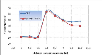
Figure (8) Velocity distribution (measured & CFD) (Scenario 3)

Some of graphical comparisons are presented here just to ve- rify this mathematical model. Figure (9) represent the free sur- face profile along longitudinal section of the flume to measure the depth of flow.

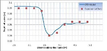
Figure (9) free surface flow model by CFD and experimental data

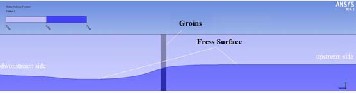
Figure (10) free surface flow model by CFD
Brefilly, from all these comparison, since the values of longi- tudinal velocity profile and water depth achieved from the CFD model were compared with experimental data. As illu- strated in all the tables, the CFD model was in good agreement with experimental result ,but in some points, the result of CFD model have some difference with experimental results.
3. CFD Modeling Overview:
In CFD calculations, there are three main steps.
• Pre-Processing
• Solver Execution
• Post-Processing

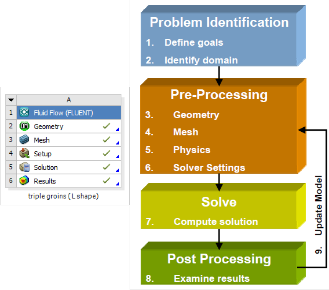
Pre-Processing is the step where the modeling goals are determined and computational grid is created. In the second step numerical models and boundary conditions are set to start up the solver. Solver runs until the convergence is reached. When solver is terminated, the results are examined which is the post-processing part. Figure (11) steps for CFD modeling

Figure (11) Steps for CFD modeling

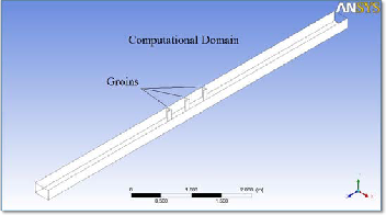
Model size is the computational domain where the solution is done figure (12). It is important to build it as small as possible to prevent the model to be computationally expensive. On the other hand it should be large enough to resolve all the fluid flow domains (water and air) characteristics around the Groins.
Figure (12) Computational domain for present work.

International Journal of Scientific & Engineering Research Volume 5, Issue ŗŘǰȱ ȬŘŖŗŚȱȱ

ISSN 2229-5518

147

Boundary conditions: pressure inlet, and pressure outlet are used to model the entire flow and exist through the do- main. These boundary conditions are more conformal to model multiphase flow. Bottom, side wall of the domain, and groins are model as a wall with no-slip conditions. Top of the domain are model as a symmetry condition to represent at- mosphere pressure. Figure (13) represent boundary conditions used in the model.

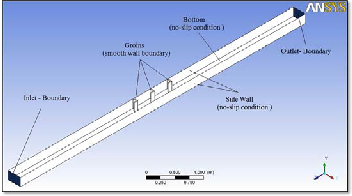
Figure (13) Computational domain and boundary conditions for CFD model

4. Mesh independent solution

One more important aspect to reduce the error in CFD calcula-
tions is to have a grid-independent solution. Grid must be fine
enough to capture all flow features and analysis results must not change when the models are run with finer meshes. If the results are changing as the numbers of cells used are in- creased, then finer mesh should be created for grid- independency. (Emre, 2004)
It is desirable to use fine meshes for flow computations in or- der to capture detailed flow features such as eddies and veloc- ity shears. Meshes were generated on the basis of a number of criteria :( Sahar, 2012)

First, meshes are fine enough in order to resolve rapid spatial variations in the velocity fields, especially near Groins boundaries. This requirement is satisfied by performing infla- tion on meshes adjacent to solid walls where eddies and veloc- ity shear are expected to appear Figure (14).

Second, the structure of meshes used for flow computations must not affect the computational results. In other words, the model results produced should be independent of the configu- rations of the meshes used.

Third, the total number mesh points must not be excessively larger, resulting in prohibitively high computation cost. An excessively large number of mesh points will also create diffi- culties in the post processing of model output.

The strategies used in the present work to satisfy this re-
quirement were to several mesh systems of progressive fine
sizes (52460, 419680,781769 and 1007829 elements) and to carry
out model runs using the different meshes under identical
flow conditions. The independence of the computed flow field
for these runs was verified through comparisons of the results
among these runs.

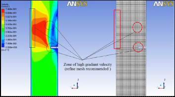
Figure (14) Zone of high gradient velocity to capture refine mesh zone.

Figure (15) present velocity distribution and mesh under iden- tical flow conditions for four meshes system.

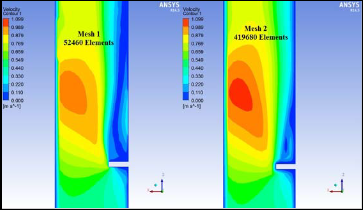
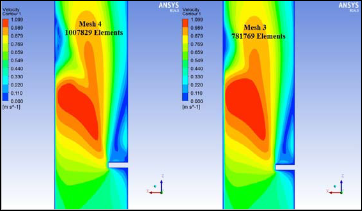
Figure (15) Velocity distribution for different meshes strateg- ist.

A mesh independence study was conducted for assessing the grid sensitivity of the results. Four mesh systems, Mesh-1 (coarse), Mesh-2 (medium) Mesh-3 (fine), and Mesh-4 (refine mesh) consisting of 52460, 419680,781769 and 1007829 ele- ments in total, respectively, were used to examine the effect of the mesh size on the accuracy of the numerical results.

International Journal of Scientific & Engineering Research Volume 5, Issue ŗŘǰȱ ȬŘŖŗŚȱȱ

ISSN 2229-5518

148

It can be seen that, the velocity profile are still change ac- cording to increases the mesh density through the Mesh-1, Mesh-2, and Mesh-3. After that a grid-independent solution have been reach it Mesh-4 as relative comparison not acceded
0.5% as maximum difference
Figures (16) and (17) represent another comparison for
grid-independent at free surface

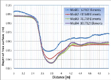
Figure (16) Free surface profile for different mesh system

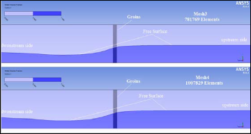
Figure (17) free surface profile for different mesh system (side view)
It can be seen that, depth of free surface are still change according to increases the density of mesh for three mesh sys- tem. This shows that Mesh-3 781769 cells are enough for the
models to be grid independent.

5. Mesh Adaption method:

One of the advantages to used high gradient adaptation method is to refine mesh near the boundary of high gradient velocity, although a mesh must be refined where flow features change rapidly, sometimes the location cannot be determined during the initial meshing.
In the present work, gradient adoptions method had been used to refine mesh localised selected by regions where pa- rameters (high gradient velocity) change rapidly. Figures (18) and (19) present level of adaption on marked cells.

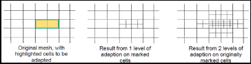
Figure (18) Method of adaption for different levels on marked cells

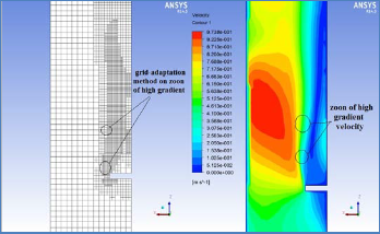
Figure (19) Grid-adaptation details for the present work to refine mesh

6. Governing equation and solver setting:

6.1 Solver

There are two kinds of solvers available in (ANSYS 14.5.7, FLUENT Code):

• Pressure based solver

• Density based solver

The pressure-based solvers: take momentum and pressure (or
pressure correction) as the primary variables

Density-Based Coupled Solver: Equations for continuity,

momentum, energy and species (if required) are solved in vec-
tor form.
The pressure-based solver had been used in the present CFD
model for many reasons: is applicable for a wide range of flow
regimes from low speed incompressible flow to high-speed
compressible flow. Requires less memory (storage). Allows
flexibility in the solution procedure. (ANSYS 14.5.7, FLUENT

Code):

International Journal of Scientific & Engineering Research Volume 5, Issue ŗŘǰȱ ȬŘŖŗŚȱȱ

ISSN 2229-5518

149

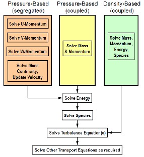
Figure (20) Flow chart algorithms for pressure-based solvers

(ANSYS.2010b)

6.2 Governing Equations of CFD:

The cornerstone of computational fluid dynamics is the
fundamental governing equations of fluid dynamics, the con- tinuity, momentum and energy equations. These equations speak physics.
The conservation of mass, momentum and energy,
these equations combine to form the Navier-Stokes equations,
which are a set of partial differential equations that cannot be solved analytically except in a limited number of cases. How- ever, an approximate solution can be obtained using a discreti- sation method that approximates the partial differential equa- tions by a set of algebraic equations. There are a variety of techniques that may be used to perform this discretisation; the most often used are the finite volume method, the finite ele- ment method and the finite difference method. The resulting algebraic equations relate to small sub-volumes within the flow, at a finite number of discrete locations.

6.2.1 Conservation of mass:

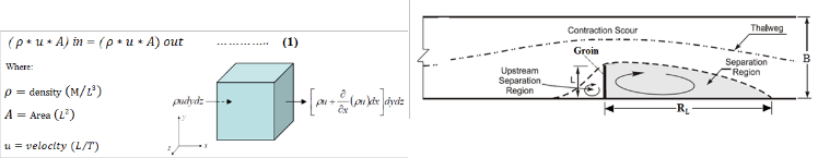
Equation (1) shows the principle conservation of mass states that in any time interval of and for any control volume, the volume of mass entering must equal the volume of mass leav- ing.

Since the averages of velocity fluctuations are zero, resultant equation becomes the Reynolds-averaged equation of continu- ity.

6.2.2 Conservation of momentum:

The momentum equations for open channel flow can be writ-

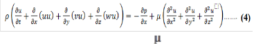
ten as:
Where : ρ = density of water, t = time, = dynamic viscosity of water, and p = pressure field
On the left hand side of the above equations, the first term is a transient term that describes the local rate of change of the velocity, and the remaining three terms are convection terms. On the right side of the equations, there are a pressure gra- dient term, and three molecular diffusion terms. It is assumed that the fluid is incompressible, and therefore, the density of water is constant with respect to time and space.

7. Parametric Study :

After it has been verified the CFD model to represent the va-
riety of complex flow around groins in the previous part, pa-
rametric study on most important design parameters will be
discuses extensively in this part of analysis.
In order to explain the effect of all these parameters, some
off physical term and variables had been adopted as a rule for comparison between the varies cases and conditions, these
variables are

Reattachment length (RL ) : it is a distance where the sepa- rated flow reattaches side wall of river downstream of groins,

figure (21)
Maximum bed shear stress (max ): The analysis of shear stress
field at the channel bed presents a particular interest for
studying the sediment and scour around the groins. The crite-
rion of starting motion for practical place at the bottom is gen-
erally estimated from critical bed shear stress constituting
threshold (Ouillon and Le Guennce 1996).

Separation region (SR): represent the max width of separated zone on groins reach.

Maximum velocity (Vmax) :which mean the ultimate velocity cause be groins structures.

Figure (21). Typical parameters for flow around groins.

International Journal of Scientific & Engineering Research Volume 5, Issue ŗŘǰȱ ȬŘŖŗŚȱȱ

ISSN 2229-5518

7.1 LENGTH OF GROINS (LG):

150

One of the most important design parameters it’s the length of groins Lg, The length of a groin is based on the length neces- sary to shift current away from the bank. Gupta et al (1969) developed the following equation to determine length of spur dike:

Where:

Lg = length of Groins

B = channel width

n = empirical coefficient from graph in paper

F = Froude number.

In other word, Length should not be less than that required to keep the scour hole formed at the nose away from the bank.
In this part of analysis, straight groin with different length ratios or contraction ratio (Lg/B) (groin length divided by channel width) varied from 10, 15, 20, 25 and 30%, had been studied to illustrated the effect of groins length on the flow pattern.
The following figures (22),(23),(24),(25), and (26) illustrated the velocity profile, and bed shear stress for different cases.
From these figures, it can be observed that the velocity in-
creases with the increase groins length ratio, and it is fact. Also
contraction ratio will increases the value of shear stress force on the bed of channels

Table (4) Represent calculated values of velocity increments, bed shear stress, thalweg offset, and reattachment length for different (Lg/B)

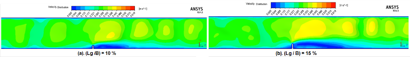
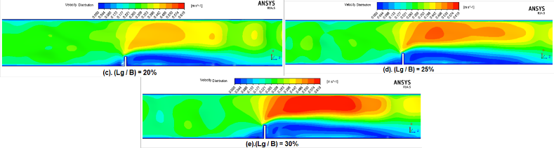
Figure (22) Velocity distribution at free surface for different length ratio

Figure (23) Net velocity difference between 30% and 10 % (Lg/B).

International Journal of Scientific & Engineering Research Volume 5, Issue ŗŘǰȱ ȬŘŖŗŚȱȱ

ISSN 2229-5518

151

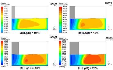
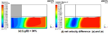
Figure (24) Velocity profile at cross section downstream of groins.

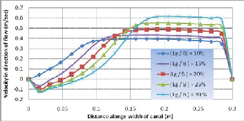
Figure (25) Velocity profile through cross section downstream of groins.

Figure (26) Eddy motion through cross section downstream of groins.

7.2 ORIENTATION OF GROINS:

Groin orientation (defined as angle between downstream bank and axis of Groins) has been determined historically by design experience. ( Klump, et al . 1992). In general, groins may be oriented upstream, downstream or perpendicular to the flow.
Five different angles of installations (measured from down- stream axis) were examined to investigate its effect on flow pattern in an open channel. The details are presented as fol- lowing.
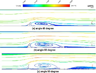
The following figures (27),(28), and (29) illustrated the velocity profile, and stream line flow for different groins orientations. Figure (27),(28) shows that velocity distribution , and shear stress are directly proportional with the angle of groins till it reach peak values at 90° , and inversely proportionally with angle more than 105°.
Figure (29) shows that, stream line of separated region are directly proportional with the angle of groins till it reaches peak values at 90°, and inversely proportionally with angle more than 105°. Also angle more than 105 will lead to erodible the upstream side of groins as showing in figure (5.13e).
Table (5) Represent calculated values of velocity increments, bed shear stress, thalweg offset, and reattachment length for groins orientations.

As seen in these figures and table (5), the maximum reat- tachment length received with groins orientation 90° for 13 times of groins length, and minimum at 45°, the maximum shear stress accrued at groins installation angle 90° which probably will lead to scour around groins nose.
Results also declared that with an increase in groins installa- tion angle, the location of the return flow zone centre shifts away from the channel sidewall.
According to data mentioned in table (5), groins orientation on downstream reduces scour (shear stress) at the end of the groins by 50%.

International Journal of Scientific & Engineering Research Volume 5, Issue ŗŘǰȱ ȬŘŖŗŚȱȱ

ISSN 2229-5518

152

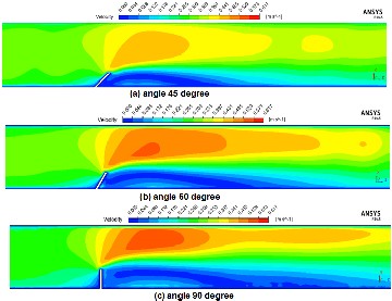
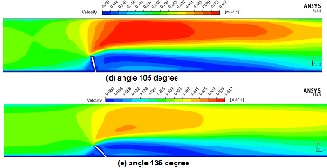
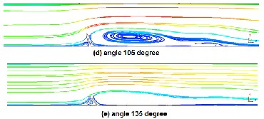
Figure (27) velocity distribution at free surface for different orientations

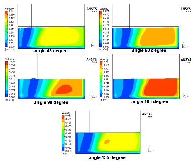
Figure (28) velocity profile through cross section down- stream of groins

Figure (29) Stream line at free surface colored by velocity for different groins orientations

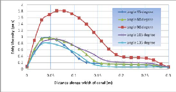
Figures (30) and (31) illustrate the velocity profile, and eddy motion viscosity through cross section downstream of groins for different groins angle.

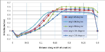
Figure (30) velocity distribution for different groins orien- tations.

International Journal of Scientific & Engineering Research Volume 5, Issue ŗŘǰȱ ȬŘŖŗŚȱȱ

ISSN 2229-5518

153

[5] ANSYS. ANSYS FLUENT 12.0 User’s guide. ANSYS Inc., 13 edition, April

2009a

[6] Klump, Cassie and, Baird, Drew, "Recent Criteria for Design of Groins" (1992). U.S. Bureau of Land Management Papers. University of Nebraska - Lincoln. Paper 29. http://digitalcommons.unl.edu/usblmpub/29

[7] Sahara. N, (2012).” CFD Modelling of Turbulent Flow in Open Channel Expansions” MSC Thesis. Department of Building, Civil, and Environmental Engineering at Concordia University Montreal,

Quebec, Canada

Figure (31) Eddy viscosity on cross section downstream of groins for different groins orientations.

8. CONCLUSION

The following main conclusions were obtained based on the results of Computational Fluid Dynamic model (CFD) for flow around groins.
Computational Fluid dynamic model (CFD) provide an effec- tive way to understand the details of the complex flow around groins and scour processes, some of which are very difficult to resolve if not impossible with only experimental methods. Comparisons between the results of CFD model with the re- sults of laboratory work explain excellent agreement for cases simulated through this research. It was found that the multi- phase volume of fluid (VOF) method along with the selected turbulence models can well describe the physics of the open channel flow ( free surface flow, water air interaction ).

Groins constructed in a channel causes changes in the velocity,

bed shear stress and pressure fields resulting in flow that is three- dimensional in character. Eddies with large velocities are gener- ated downstream of groins.

The reattachment length (RL) is covers about 12-13 times the length of grins. Reattachment length (RL) can provide helpful advice for the groins installation interval. It was found that, groins with (Lg/B) more than 20% will have a significant effects on the opposite bank of channel and will increased the velocity and shear stress by 76, and 99 % respectively A groin with (Lg/B) less than 10% does not have a clear effect on the flow characters and causes to lead the scour near the bank, which is not desirable for stabilize the bank.The maximum bed shear stress, and reattachment length will accrued at groins installation angle 90° which probably will lead to scour around groins nose. Groins oriented either normal to the flow or slightly down- stream for best performance.

REFERENCES

[1] ANSYS (2010b)“ANSYS CFD Solver Theory Guide”. Release 13.0, ANSYS, Inc.

[2] ANSYS (2010a) “ANSYS -FLUENT user’s guide”. Release 13.0, ANSYS, Inc

[3] ANSYS.14.5.7. ANSYS- FLUENT Theory Guide. ANSYS Inc., 13 editions, November 2010

[4] ANSYS. ANSYS FLUENT 12.0 Meshing Help. ANSYS Inc., release 12.1 edi-

tions, November 2009c.

[8] Emre Özturk, 2004 , “ CFD Analyses of Heat Sinks for CPU Cool- ing with Fluent ”, MSc Thesis , Middle East Technical University.

[9] Carling, P. A., Kohmann, F., and Golz, E.: (1996). “River Hydraulics, Sediment Transport and Training Works”: their ecological rele- vance to European rivers, Archiv. Hydrobiol. Suppl., Vol. 113, No.10, pp. 129-146.

[10] Shields Jr., F.D., Cooper, C.M. & Knight S.S. (1995). “Experiment in

Stream Restoration”. Journal of Hydraulic Engineering, ASCE,

121(6): 494-502.

[11] Teraguchi, H., (2011). “Study on Hydraulic and Morphological Char- acteristics of River Channel with Groin Structures”, Ph. D. Thesis, Kyoto University