Inventory Model for Deteriorating Items Having Two Component Mixture of Pareto Lifetime and Selling Price Dependent Demand

International Journal of Scientific & Engineering Research, Volume 5, Issue 7, July-2014 254

ISSN 2229-5518

Vijayalakshmi. G, Srinivasa Rao. K and Nirupama Devi. K

Abstract — In this paper, we develop and analyses an inventory model with the assumption that the life time of commodity is random and f ollows two component mixture of Pareto distribution. It is also assumed that the demand is a function of selling price. Using the differential difference equations, the instantaneous state of inventory is derived. W ith suitable cost considerations, the total cost function per a unit time and the profit rate function are obtained. Sensitivity analysis is also carried out for this model. This model is useful in practical situations like food processing industries, market yards dealing with agricultural products.

Key words — demand, deteriorating items, life time, mixture distributions, Pareto distribution, selling price.

——————————  ——————————

1 INTRODUCTION

NVENTORY modeling is a prerequisite for developing the optimal ordering and pricing policies in several places such as ware houses, market yards, production processes, cargo handling. When one is concerned with the inventory control, it is essential to identify two important factors namely, the nature of the goods procured and the nature of the de- mand. When we consider the nature of procurement, we have to consider life time of the commodity along with the demand pattern (K.Srinivasa Rao et.al [9], K.V Subbiah et.al [14]). De- cay or deterioration of physical goods while in stock is a common phenomenon. . Pharmaceuticals, food, vegetables and fruits are a few examples of such items. Taking this into consideration, deteriorating inventory models have been widely studied in recent years. The analysis of decaying in- ventory problems began with Ghare, P.M and Schrader,G.F [2] who developed an economic order quantity model with con- stant rate of decay (exponential life time). Covert R.P and Phil- ip, G.C [1] extended this model and obtained an economic order quantity model for a variable rate of deterioration by assuming a two parameter Weibull distribution. Extensive reviews of research literature on the deteriorating items are provided by Raafat, F [7], Goyal S.K. and Giri B.C [3] and Liao.
et al [6].
Very little work has been done in perishable invento- ry models with heterogeneous life time of the commodity. Several authors have studied the perishable inventory models with the assumption that the life time of the commodity is random and follows a probability distribution having the ho- mogenous nature.
However in some situations prevailing at places like

————————————————

• Vijayalakshmi. G, Researche Scholar

E-mail: gullipallivijaya@gmail.com

• Srinivasa Rao. K, Professor, E-mail: ksraoau@yahoo.co.in

• Nirupama Devi. K, Professor,

E-mail: knirupamadevi@gmail.com

Dept.of Statistics, Andhra University, Visakhapatnam, India.

fruit and vegetable markets, food processing industries, photo
chemicals, pharmaceutical industries, the stock on-hand is
procured from various sources for the same type of items. Even though the nature of the item does not differ, there will be some inherent variation due to the source from which they are procured. So the efficiency of the inventory model heavily depends upon the probability distribution ascribed to the life time of the commodity under consideration. In general the stock on-hand with respect to the perishability can be consid- ered as a heterogeneous population consisting of two types of life times viz., shorter and longer life times. When the items are mixed in stock, it is difficult to isolate each item with re- spect to their life time. So in order to associate suitable proba- bility model to the life time of the commodity one has to con- sider the mixture of distributions (Srinivasa Rao et al [10].
Hence in this paper, we consider the life time of the
commodity is random and follows a two component Pareto
mixture of distributions. The Pareto life time distribution is
capable of characterizing age dependent rate of deterioration. The Pareto distribution is extensively used in reliability and life testing experiments.
In addition to the life time of the commodity, another important factor that influences the inventory system is the
nature of the demand. Several demand patterns were used for analyzing the inventory situations (Srinivasa Rao et al [10]). Among all these demand patterns selling price dependent demand gained lot of importance in developing and analyzing the inventory models (Lakshmi Narayana et al. [5], Srinivasa Rao et al. [11], Sridevi et al [8], U.M.Rao et al [13], Essey et al. [4]). In this article also it is assumed that the demand is a line- ar function of selling price.
Using the differential difference equations the instan- taneous state of inventory is derived with suitable cost consid- erations. The total cost function per a unit time and the profit
rate function are derived. Through numerical illustration the sensitivity of the model with respect to the cost is also studied. This model is much useful for analyzing inventory situations arising at the food processing industries, market yards dealing with agricultural products.

International Journal of Scientific & Engineering Research, Volume 5, Issue 7, July-2014 255

ISSN 2229-5518

2 INVENTORY MODEL FOR DETERIORATING ITEMS WITH SELLING PRICE DEPENDENT DEMAND

Consider an inventory system for deteriorating items in which the life time of the commodity is random and follows two component mixture of Pareto distribution with probabil- ity density function of the form

𝑓(𝑡) = 𝛼𝛽1 θ𝛽1 𝑡−(𝛽1 +1) + (1 − 𝛼)𝛽2 θ𝛽2 𝑡 −(𝛽2 +1) 𝑡 ≥ θ

π: Shortage cost per unit per unit time

s: Selling price of a unit

𝝀(𝒔): Demand rate
In this model the stock level (initial inventory) is Q at time
𝑡 = 0. The stock level decreases during the period (0, θ) due
to demand and due to demand and deterioration during the
period (θ, t1 ) . At time t1 inventory reaches zero and back or- ders accumulate during the period (t1, T). Let 𝐼(𝑡) be the inventory level of the system at time t (0 ≤ t ≤ T)
The distribution function of t is
θ 𝛽1

θ 𝛽2

𝐹(𝑡) = 𝛼 �1 − �𝑡 �

� + (1 − 𝛼) �1 − �𝑡 � �
The mean life time of the commodity is
𝛽1 θ
𝛽2 θ
Fig.1 : Schematic diagram representing the inventory level

µ = 𝛼 (𝛽

− 1) + (1 − 𝛼) (𝛽
− 1) 𝑡 ≥ θ, 𝛽1 > 1, 𝛽2 > 1
The differential equations governing the instantaneous state of
The variance of life time of the commodity is
𝐼(𝑡) over the cycle length T are
𝑉𝑉𝑉(𝑡) = 𝛼

𝛽1 θ2
𝛽1 − 2
+ (1 − 𝛼)

𝛽2 θ2
𝛽2 − 2

𝑑
𝑑𝑡
𝐼(𝑡) = −𝜆(𝑠) 0 ≤ 𝑡 ≤ 𝜃 (3.1.1)

𝛽1 θ
𝛽2 θ 2
𝑑

𝐼(𝑡) + ℎ(𝑡)𝐼(𝑡) = −𝜆(𝑠) 𝜃 ≤ 𝑡 ≤ 𝑡
(3.1.2)
− �𝛼 (𝛽
− 1) + (1 − 𝛼) (𝛽
− 1)�
𝑡 ≥ θ, 𝛽1 > 2, 𝛽2 > 2
𝑑𝑡 1

𝑑
The instantaneous rate of deterioration is
𝑓(𝑡)
𝑑𝑡
𝐼(𝑡) = −𝜆(𝑠) 𝑡1 ≤ 𝑡 ≤ 𝑇 (3.1.3)
ℎ(𝑡) =

1 − 𝐹(𝑡)

𝛼𝛽1 θ𝛽1 𝑡−(𝛽1+1) + (1 − 𝛼)𝛽2 θ𝛽2 𝑡−(𝛽2 +1)

where, ℎ(𝑡) is as given in equation (2.1),with the initial con- ditions 𝐼(0) = 𝑄 , 𝐼(𝑡1) = 0.
Substituting ℎ(𝑡) given in equation (2.1) in equations (3.1.1),
(3.1.2), and (3.1.3) and solving the above differential equations,
=
1 − 𝛼 �1 − �θ�

𝛽1

𝛽2

� − (1 − 𝛼) �1 − � � �
(2.1)
the on hand inventory at time t can be obtained as

𝑡 𝑡

𝑡1

θ 𝛽1

3.1 INVENTORY MODEL FOR DETERIORATING

ITEMS WITH SELLING PRICE DEPENDENT

𝐼(𝑡) = 𝜆(𝑠) �(θ − 𝑡) + � �1 − 𝛼 �1 − � � �

𝜃

θ 𝛽2 −1

DEMAND WITH SHORTAGES

−(1 − 𝛼) �1 − � 𝑡 � ��
𝑑𝑡�
Consider an inventory system for deteriorating items in which the life time of commodity is random and follows a two com- ponent mixture of Pareto distribution with probability density of the form as given in section 2.

𝛽1

𝐼(𝑡) = 𝜆(𝑠) �1 − 𝛼 �1 − �θ�

𝑡

0 ≤ 𝑡 ≤ θ (3.1.4)

𝛽2

� − (1 − 𝛼) �1 − �θ� ��

𝑡

Assumptions:

The demand rate is a function of unit selling price

𝑡1 θ

� �1 − 𝛼 �1 − � �

𝛽1

θ

� − (1 − 𝛼) �1 − � �

𝛽2 −1

��
𝑑𝑡
Lead time is zero
Cycle length, T is unknown
Shortages are allowed

𝑡 𝑡

𝑡
θ ≤ 𝑡 ≤ 𝑡1 (3.1.5)
A deteriorated unit is lost

Notation:

Q: Ordering quantity in one cycle

𝐼(𝑡) = 𝜆(𝑠)( 𝑡1 − 𝑡 ) 𝑡1 ≤ 𝑡 ≤ 𝑇 (3.1.6)
The stock loss due to deterioration in the interval (0, 𝑡) is

A: Ordering cost

𝑡1

𝛽1

C: Cost per unit

θ

𝐿(𝑡) = 𝜆(𝑠) �(θ − 𝑡) + � �1 − 𝛼 �1 − � �
� − (1 − 𝛼)

h: Inventory holding cost per unit per unit time

θ 𝑡

International Journal of Scientific & Engineering Research, Volume 5, Issue 7, July-2014 256

ISSN 2229-5518

θ 𝛽2 −1

�1 − � 𝑡 � ��

θ 𝛽1
𝑑𝑡 − �1 − 𝛼 �1 − � 𝑡 �

θ 𝛽2
� − (1 − 𝛼) �1 − � 𝑡 � ��
𝜆(𝑠)𝜋

+
𝑇
(𝑇 − 𝑡1 ) (3.1.10)

𝑡1

θ 𝛽1

θ 𝛽2 −1

Let 𝑃(𝑡1 , 𝑇, 𝑠) be the profit rate function. Since the profit rate
function is the total revenue per unit time minus total cost per

� �1 − 𝛼 �1 − � �

𝑡

� − (1 − 𝛼) �1 − �𝑢� ��
𝑑𝑢�
unit time, we have
The stock loss due to deterioration in the interval (0, 𝑡1 ) is
𝑃(𝑡1, 𝑇, 𝑠) = 𝑠𝜆(𝑠) − 𝐾(𝑡1 , 𝑇, 𝑠) (3.1.11)
Substituting the value of 𝐾(𝑡1 , 𝑇, 𝑠) given in equation (3.1.10)

𝑡1

θ 𝛽1
in equation (3.1.11), we obtain the profit rate function as

𝐿(𝑡1 ) = 𝜆(𝑠) �(θ − 𝑡1 ) + � �1 − 𝛼 �1 − � 𝑡 �
� − (1 − 𝛼)
𝐴 𝐶𝜆(𝑠)

𝑡1

θ 𝛽2 −1

�1 − � 𝑡 � ��
𝑑𝑡� (3.1.7)

𝑃(𝑡1, 𝑇, 𝑠) = 𝑠𝜆(𝑠) − 𝑇 −

�θ + (𝑇 − 𝑡1 ) + � �1 − 𝛼

𝜃

The ordering quantity, Q in the cycle length 𝑇 is
𝑄 = 𝐿(𝑡1 ) + 𝜆(𝑠)𝑡1 + 𝜆(𝑠)(𝑇 − 𝑡1 )
θ
�1 − �𝑢
ℎ𝜆(𝑠) θ

𝛽1

�
θ
� −(1 − 𝛼) �1 − �𝑢

𝑡1

𝛽2 −1

� ��
θ
𝑑𝑢�

𝛽1

− � �(θ − 𝑡) + � �1 − 𝛼 �1 − � �
� − (1 − 𝛼)

𝑡1

θ 𝛽1
𝑇 0 θ 𝑢

= 𝜆(𝑠) �θ + (𝑇 − 𝑡1 ) + � �1 − 𝛼 �1 − � � �

𝜃

θ 𝛽2 −1

ℎ𝜆(𝑠)

𝑡1

θ 𝛽1

θ 𝛽2 −1

−(1 − 𝛼) �1 − � 𝑡 � ��
𝑑𝑡� (3.1.8)

�1 − �𝑢� ��
𝑑𝑢� 𝑑𝑡 −

� ��1 − 𝛼 �1 − � � �
𝑇 𝜃 𝑡
Let 𝐾(𝑡1 , 𝑇, 𝑠) be the total cost per unit time. Since the total cost is sum of the set up cost, cost of the units, the inventory hold-
−(1 − 𝛼) �1 − �

θ 𝛽2
𝑡 �

𝑡1

�� 1 − 𝛼 �1 − �

𝑡

θ 𝛽1
𝑢� �
ing cost, the shortage cost, 𝐾(𝑡1 , 𝑇, 𝑠) becomes
−(1 − 𝛼) �1 − �

θ 𝛽2 −1

� ��
𝑑𝑢 � 𝑑𝑡 +

𝜋
(𝑇 − 𝑡1 ) 2 (3.1.12)
𝐴 𝐶𝑄 ℎ θ

𝑡1

𝜋 𝑇
𝑢 2𝑇

𝐾(𝑡1 , 𝑇, 𝑠) = 𝑇 +

+ �� 𝐼(𝑡)𝑑𝑡 + � 𝐼(𝑡)𝑑𝑡� + � −𝐼(𝑡)𝑑𝑡
𝑇 𝑇 𝑇

0 θ 𝑡1

(3.1.9)

3.2 OPTIMAL PRICING AND ORDERING POLICIES OF THE MODEL

Substituting the values of 𝐼(𝑡) and Q given in equations (3.1.4),
(3.1.5), (3.1.6) and (3.1.8) in equation (3.1.9), we obtain
𝐾(𝑡1 , 𝑇, 𝑠) as
In this section we obtain the optimal policies of the inventtory system developed in section 3.1. The conditions for obtaining optimality are
𝐴 𝜆(𝑠)𝐶

𝑡1

θ 𝛽1

𝐾(𝑡1 , 𝑇, 𝑠) = 𝑇 +

𝑇 �θ + (𝑇 − 𝑡1 ) � �1 − 𝛼 �1 − �𝑢� �

𝜕

𝜕𝑡1

𝑃(𝑡1 , 𝑇, 𝑠) = 0 ;

𝜕

𝜕𝑇

𝑃(𝑡1 , 𝑇, 𝑠) = 0;

𝜕

𝜕𝑠

𝑃(𝑡1 , 𝑇, 𝑠) = 0;

θ 𝛽2 −1

𝜆(𝑠)ℎ 𝜃

𝑡1

𝜕

2 𝑃(𝑡1 , 𝑇, 𝑠)

𝜕

𝑃(𝑡1 , 𝑇, 𝑠)

𝜕

𝑃(𝑡1 , 𝑇, 𝑠)

−(1 − 𝛼) �1 − �𝑢� ��
𝑑𝑡� +
� �(θ − 𝑡) + � �1 − 𝛼
𝑇
� 𝜕𝑡1
𝜕𝑡1 𝜕𝑇
𝜕𝑡1 𝜕𝑠 �
θ
�1 − �𝑢�

𝛽1

θ
� − (1 − 𝛼) �1 − �𝑢�

𝛽2 −1

��

𝑑𝑢� 𝑑𝑡 +

𝜆(𝑠)ℎ
𝑇
𝐷 =
𝜕

𝜕𝑇𝜕𝑡1
� 𝜕
𝜕𝑠𝜕𝑡1
𝑃(𝑡1 , 𝑇, 𝑠)
𝑃(𝑡1 , 𝑇, 𝑠)
𝜕2

𝜕𝑇 2 𝑃(𝑡1, 𝑇, 𝑠)
𝜕
𝜕𝑠𝜕𝑇 𝑃(𝑡1 , 𝑇, 𝑠)
𝜕

𝑃(𝑡1 , 𝑇, 𝑠) < 0
𝜕𝑇𝜕𝑠
𝜕2 �
𝜕𝑠2 𝑃(𝑡1 , 𝑇, 𝑠)

𝑡1

θ 𝛽1

θ 𝛽2 −1

� �1 − 𝛼 �1 − � 𝑡 �
� − (1 − 𝛼) �1 − �𝑢� ��
𝑑𝑢� 𝑑𝑡
where D is the determent of Hessian matrix
Differentiating (3.1.12) with respect to 𝑡1and equating to zero,

𝑡1

θ 𝛽1

θ 𝛽2 −1

we get

� �1 − 𝛼 �1 − � �

𝑡

� − (1 − 𝛼) �1 − �𝑢� ��
𝑑𝑢 � 𝑑𝑡

θ
𝑐 �1 − �1 − 𝛼 �1 − �𝑡 �

𝛽1

θ
� − (1 − 𝛼) �1 − �𝑡 �

𝛽2

−1

��

International Journal of Scientific & Engineering Research, Volume 5, Issue 7, July-2014 257

ISSN 2229-5518

θ θ 𝛽1

θ 𝛽2 −1

𝜋
− (𝑇 − 𝑡1 )2 = 0 (3.2.3)

−ℎ � �1 − 𝛼 �1 − �𝑡 �

� − (1 − 𝛼) �1 − �𝑡 � ��
𝑑𝑡
2𝑇

𝑡1

θ 𝛽1

θ 𝛽2
Solving equations (3.2.1), (3.2.2) and (3.2.3) simultaneously, we
obtain the optimal cycle length, 𝑇 ∗ , time at which shortages
occur 𝑡1 ∗ and optimal selling price, 𝑠 ∗.

−ℎ � ��1 − 𝛼 �1 − � 𝑡 �

� − (1 − 𝛼) �1 − � 𝑡 � ��
The optimal ordering quantity, 𝑄∗ is obtained by substituting

θ 𝛽1
�1 − 𝛼 �1 − � 𝑡 �

θ 𝛽2
� − (1 − 𝛼) �1 − � 𝑡 �

−1

�� 𝑑𝑡
the optimal values of 𝑡1 , T and s in equation (3.1.8).
𝑄∗ = 𝜆(𝑠∗ ) �θ + (𝑇 ∗ − 𝑡1 ∗ )
−𝜋(𝑇 − 𝑡1 ) = 0 (3.2.1)

𝑡1 ∗

θ 𝛽1

θ 𝛽2 −1

Differentiating (3.1.12) with respect to T and equating to zero,
we get

+ � �1 − 𝛼 �1 − � 𝑡 �

� − (1 − 𝛼) �1 − � 𝑡 � ��
𝑑𝑡�
(3.2.4)
𝐴 t1
θ 𝛽1

𝜆(𝑠) − C �(𝑡1 − θ) + � �1 − 𝛼 �1 − �𝑢�
� − (1 − 𝛼)

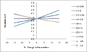
3.3 SENSITIVITY ANALYSIS

The sensitivity analysis is carried to explore the effect of

θ 𝛽2 −1 𝜃

𝑡1

θ 𝛽1

changes in model parameters and costs on the optimal values

�1 − �𝑢� ��
𝑑𝑢� + ℎ � �(θ − 𝑡) + � �1 − 𝛼 �1 − �𝑢� �
of time at which shortages occur, the cycle length, selling

0 𝜃

θ 𝛽2 −1

price, ordering quantity. by varying each parameter ( -15%, -
10%, -5%, 0%, 5%, 10%, 15% ) at a time for the model under

𝑡1

−(1 − 𝛼) �1 − �𝑢� ��
θ 𝛽1
𝑑𝑢� 𝑑𝑡
θ

𝛽2 −1

study. The results are presented in Table 1. The relationship
between the parameters and the optimal values are shown in

Fig 2.

Table 1

+ℎ � �� 1 − 𝛼 �1 − �𝑢�

� − (1 − 𝛼) �1 − �𝑢� ��
𝑑𝑢

Sensitivity analysis of the model – with shortages

𝜃 𝑡

θ 𝛽1
θ 𝛽2

�1 − 𝛼 �1 − � 𝑡 �

� − (1 − 𝛼) �1 − � 𝑡 �
�� dt
+𝜋(T2 − 𝑡1 2 ) = 0 (3.2.2)
Differentiating (3.1.12) with respect to s and equating to zero,
we get
𝑠 +

𝜆(𝑠)
𝜆′(𝑠)

𝑐
− 𝑇 �θ + (𝑇 − 𝑡1 )

𝑡1

θ 𝛽1

θ 𝛽2 −1

+ � �1 − 𝛼 �1 − �𝑢�

� − (1 − 𝛼) �1 − �𝑢� ��
𝑑𝑢�
ℎ θ 𝑡1
θ 𝛽1

− � �(θ − 𝑡) + � �1 − 𝛼 �1 − � � �
𝑇 0

θ 𝑢

θ 𝛽2 −1

−(1 − 𝛼) �1 − �𝑢� ��
𝑑𝑢 � 𝑑𝑡

ℎ 𝑡1
− � ��1 − 𝛼 �1 − �
𝑇 θ
θ 𝛽1
𝑡 �
� − (1 − 𝛼) �1 − �

θ 𝛽2
𝑡 � ��

𝑡1

θ 𝛽1

θ 𝛽2 −1

� �1 − 𝛼 �1 − � �

𝑡

� − (1 − 𝛼) �1 − �𝑢� ��
𝑑𝑢 � 𝑑𝑡

International Journal of Scientific & Engineering Research, Volume 5, Issue 7, July-2014 258

ISSN 2229-5518

As the ordering cost A increases the optimal time at
which shortages occur 𝑡1 ∗, the optimal cycle length 𝑇 ∗, opti-
mal selling price 𝑠∗ , and optimal quantity 𝑄∗ , are increasing

and profit per unit time 𝑃∗, is decreasing. As the cost per unit
C increases, the optimal time at which shortages occur 𝑡1 ∗, the
optimal cycle length 𝑇 ∗, and profit per unit time 𝑃∗, and
optimal ordering quantity 𝑄∗ are decreasing and optimal sell-
ing price 𝑠∗ , is increasing.
As the holding cost h increases the optimal time at
which shortages occur 𝑡1 ∗, and profit per unit time 𝑃∗, are decreasing and the optimal cycle length 𝑇 ∗, optimal selling price 𝑠 ∗, optimal ordering quantity 𝑄∗ are increasing.
As the shortage cost π increases, the optimal time at
which shortages occur 𝑡1 ∗ increases and optimal cycle length

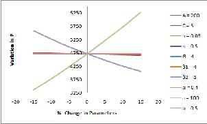
𝑇 ∗, optimal selling price 𝑠∗ , optimal profit per unit time 𝑃∗,
optimal ordering quantity 𝑄∗ are decreasing. As the scale
parameter 𝜃 increases, the optimal time at which shortages
occur 𝑡1 ∗, the optimal cycle length 𝑇 ∗, and profit per unit time
𝑃∗, and optimal ordering quantity 𝑄∗ are decreasing and op-
timal selling price 𝑠∗ , is decreasing.
As the shape parameter 𝛽1 increases, optimal time
at which shortages occur 𝑡1 ∗, the optimal cycle length 𝑇 ∗, op-
timal selling price 𝑠∗ , optimal profit per unit time 𝑃∗, optimal
ordering quantity 𝑄∗ are decreases. As the shape parameter
𝛽2 increases, optimal time at which shortages occur 𝑡1 ∗, the
optimal cycle length 𝑇 ∗, optimal selling price 𝑠∗ , optimal prof-
it per unit time 𝑃∗, optimal ordering quantity 𝑄∗ are de-

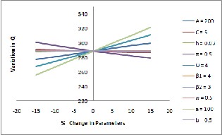
creases.
As the mixing parameter 𝛼 increases, optimal time at which shortages occur 𝑡1 ∗, the optimal cycle length 𝑇 ∗, opti- mal selling price 𝑠∗ , optimal profit per unit time 𝑃∗, optimal ordering quantity 𝑄∗ are decreasing. As the demand parame- ter a increases, the optimal time at which shortages occur 𝑡1 ∗, the optimal cycle length 𝑇 ∗, are decreases and optimal selling price 𝑠 ∗, optimal profit per unit time 𝑃∗, and optimal order- ing quantity 𝑄∗ are increasing. As the demand parameter ‘ b ’ increases, the optimal time at which shortages occur 𝑡1 ∗, the optimal cycle length 𝑇 ∗, are increasing and optimal selling price 𝑠 ∗, optimal profit per unit time 𝑃∗, and optimal order- ing quantity 𝑄∗ are decreasing.

Fig 2: Relationship between optimal values and parameters with shortages

International Journal of Scientific & Engineering Research, Volume 5, Issue 7, July-2014 259

ISSN 2229-5518

4.1 INVENTORY MODEL FOR DETERIORATING

ITEMS WITH SELLING PRICE DEPENDENT

𝑇 θ 𝛽1

θ 𝛽2 −1

DEMAND WITHOUT SHORTAGES

In section 3, the inventory model for deteriorating items with selling price dependent demand and as a function of selling

� �1 − 𝛼 �1 − � �

𝑡

� − (1 − 𝛼) �1 − � 𝑡 �
�� 𝑑𝑡�
0 ≤ 𝑡 ≤ 𝑇
price and with shortages is discussed. In this section the model without shortages is developed and analyzed. For developing
the model, we assume that 𝜋 → ∞ and 𝑡1 → 𝑇.
In this model the stock level (initial inventory) is Q at
time 𝑡 = 0. The stock level decreases during the period (0, θ)
The stock loss due to deterioration in the cycle of length T is
𝐿(𝑇) = 𝜆(𝑠) �(θ − 𝑇)
due to demand and due to deterioration and demand during 𝑇
θ 𝛽1

θ 𝛽2 −1

the period (θ, T). At time 𝑇 inventory reaches zero.
The differential equations governing the instantaneous state of

+ � �1 − 𝛼 �1 − � 𝑡 �

� − (1 − 𝛼) �1 − � 𝑡 � ��
� 𝑑𝑡
𝐼(𝑡) over the cycle length T are
𝑑
The ordering quantity, Q in the cycle length T is
𝑑𝑡

𝑑
𝑑𝑡

𝐼(𝑡) = −𝜆(𝑠) 0 ≤ 𝑡 ≤ θ (4.1.1)
𝐼(𝑡) + ℎ(𝑡)𝐼(𝑡) = −𝜆(𝑠) θ ≤ 𝑡 ≤ 𝑇 (4.1.2)
𝑄 = 𝐿(𝑇) + 𝜆(𝑠)𝑇
= 𝜆(𝑠) �θ

𝑇

θ 𝛽1

θ 𝛽2 −1

where ℎ(𝑡) is as given in equation (2.1), with the initial condi- tions 𝐼(0) = 𝑄, 𝐼(𝑇) = 0.

+ � �1 − 𝛼 �1 − � 𝑡 �

� − (1 − 𝛼) �1 − � 𝑡 � ��
𝑑𝑡� (4.1.5)
Substituting ℎ(𝑡) given in equation (2.1) in equations (4.1.1)
and (4.1.2) and solving the differential equations, the on hand
inventory at time t can be obtained as
Let 𝐾(𝑇, 𝑠) be the total cost per unit time. Since the total cost is
sum of the set up cost, cost of the units, the inventory holding
cost, 𝐾(𝑇, 𝑠)becomes

T θ β1

𝐴 𝐶𝑄 ℎ θ 𝑇

I(t) = λ(s) �(θ − t) + � �1 − α �1 − � t � �
𝐾(𝑇, 𝑠) =

+ + �� 𝐼(𝑡)𝑑𝑡 + � 𝐼(𝑡)𝑑𝑡� (4.1.6)

θ 𝑇

𝑇 𝑇 0 θ

θ β2
−(1 − α) �1 − � t �

−1

�� dt
Substituting the values of 𝐼(𝑡) and Q given in equations (4.1.3), (4.1.4) and (4.1.5) in equation (4.1.6), we obtain 𝐾(𝑇, 𝑠) as
0 ≤ 𝑡 ≤ θ (4.1.3)
𝐴 𝐶 𝑇 θ

𝐾(𝑇, 𝑠) = + 𝜆(𝑠) �θ + � 1 − 𝛼 �1 − � �

𝛽1

�
𝐼(𝑡) = 𝜆(𝑠) �1 − 𝛼 �1 − �θ�

𝛽1

� − (1 − 𝛼) �1 − �θ�

𝛽2

��
𝑇 𝑇

𝜃 𝑢

𝛽2 −1 𝜃

𝑡 𝑡

θ
− (1 − 𝛼) �1 − � � ��

ℎ
𝑑𝑡 + 𝜆(𝑠) � �θ − 𝑡

𝑇 θ β1

θ β2 −1

𝑢 𝑇 0
� � �1 − α �1 − � �

𝑡

� − (1 − α) �1 − � t � ��
dt �

𝑇 θ

+ � �1 − 𝛼 �1 − �

θ 𝑢

𝛽1

�
θ
� − (1 − 𝛼) �1 − �𝑢

𝛽2 −1

� ��
𝑑𝑢 � 𝑑𝑡
θ ≤ 𝑡 ≤ 𝑇 (4.1.4)

ℎ 𝑇
θ 𝛽1
θ 𝛽2
The stock loss due to deterioration in the interval (0, t) is
+ 𝜆(𝑠) � ��1 − 𝛼 �1 − � �
𝑇 θ 𝑡

� − (1 − 𝛼) �1 − � 𝑡 � ��
𝐿(𝑡) = 𝐼(0) − 𝜆(𝑠)𝑡 − 𝐼(𝑡)
= 𝜆(𝑠) �(θ − 𝑡)

𝑇

� �1 − 𝛼 �1 − �

𝑡

θ 𝛽1
𝑢�
θ
� − (1 − 𝛼) �1 − �𝑢

𝛽2 −1

� ��
𝑑𝑢� 𝑑𝑡 (4.1.7)

𝑇 θ 𝛽1

θ 𝛽2 −1

Let 𝑃(𝑇, 𝑠) be the profit rate function. Since the profit rate

+ � �1 − 𝛼 �1 − � 𝑡 �

� − (1 − 𝛼) �1 − � 𝑡 � ��
𝑑𝑡
function is the total revenue per unit time minus total cost per unit time, we have

θ 𝛽1
− �1 − 𝛼 �1 − � 𝑡 �

θ 𝛽2
� − (1 − 𝛼) �1 − � 𝑡 � ��
𝑃(𝑇, 𝑠) = 𝑠𝜆(𝑠) − 𝐾(𝑇, 𝑠) (4.1.8)

International Journal of Scientific & Engineering Research, Volume 5, Issue 7, July-2014 260

ISSN 2229-5518

Substituting the values of 𝐾(𝑇, 𝑠) given in equations (4.1.7) in
(4.1.8), we get profit rate function as

θ 𝛽2 −1

−(1 − 𝛼) �1 − �𝑢� ��
𝑑𝑢� 𝑑𝑡
𝑃(𝑇, 𝑠) = 𝑠𝜆(𝑠) −
𝐴 𝐶

−
𝑇 𝑇

𝑇

𝜆(𝑠) �𝜃 + � �1 − 𝛼 �1 − �

𝜃

θ 𝛽1
𝑡 � �
θ
−𝑇 �1 − 𝛼 �1 − �𝑇

𝛽1

�
θ
� − (1 − 𝛼) �1 − �𝑇

𝛽2

�

−1

��

𝛽2 −1 𝜃

−1

−(1 − 𝛼) �1 − � 𝑡 � ��

𝑑𝑡� − 𝑇 𝜆(𝑠) � �θ − 𝑡

𝑇 𝑇

θ 𝛽1
θ 𝛽2

0 −ℎ � �� 1 − 𝛼 �1 − �𝑢�

� − (1 − 𝛼) �1 − �𝑢� ��
𝑑𝑢

𝑇 θ 𝛽1

θ 𝛽2 −1

θ 𝑡

𝛽1

𝛽2

+ � �1 − 𝛼 �1 − � �

𝛩

� − (1 − 𝛼) �1 − �𝑢� ��
𝑑𝑢� 𝑑𝑡

θ
�1 − 𝛼 �1 − � 𝑡 �
θ
� − (1 − 𝛼) �1 − � 𝑡 � ��
ℎ 𝑇

− 𝜆(𝑠) � ��1 − 𝛼 �1 − �
𝑇 θ
θ 𝛽1
𝑡 �
� − (1 − 𝛼) �1 − �

θ 𝛽2
𝑡 � ��

θ
−𝑇 �1 − 𝛼 �1 − � 𝑡 �

𝛽1

θ
� (1 − 𝛼) �1 − � 𝑡 �

𝛽2

��

𝑇 θ

𝛽1

θ 𝛽2 −1

𝛽1

𝛽2 −1

� �1 − 𝛼 �1 − � �

𝑡

� − (1 − 𝛼) �1 − �𝑢� ��
𝑑𝑢� 𝑑𝑡
(4.1.9)

θ
�1 − 𝛼 �1 − �𝑇�

θ
� (1 − 𝛼) �1 − �𝑇� ��
� 𝑑𝑡 = 0
(4.2.1)

4.2 OPTIMAL PRICING AND ORDERING POLICIES OF THE MODEL

Differentiating 𝑃(𝑇, 𝑠) given in equation (4.1.9) with respect to
s and equating to zero, we get
𝜆(𝑠)
In this section we obtain the optimal policies of the inven- tory system developed in section 4.1. To find the optimal val-
𝑠𝑇 +

𝜆′(𝑠) 𝑇

𝑇

𝛽1

𝛽2 −1

ues of T and s, we equate the first order partial derivatives of
θ
−𝑐 �θ + � �1 − 𝛼 �1 − � �

θ
� − (1 − 𝛼) �1 − � � ��
𝑑𝑡�
𝑃(𝑇, 𝑠) given in equation (4.1.9) with respect to T and s to zero
respectively. The conditions for obtaining optimality are

θ 𝑡

𝜃 𝑇

𝑡

𝛽1

𝜕 𝜕

θ
−ℎ � �θ − 𝑡 + � �1 − 𝛼 �1 − � � �

𝜕𝑇

𝑃(𝑇, 𝑠) = 0;
𝜕2

𝜕𝑠

𝑃(𝑇, 𝑠) = 0;
𝜕

0 θ 𝑢

θ 𝛽2 −1

and 𝐷 = � 𝜕𝑇 2
𝜕

𝑃(𝑇, 𝑠)
𝜕𝑇𝜕𝑠
𝜕2

𝑃(𝑇, 𝑠)
� < 0

−(1 − 𝛼) �1 − �𝑢� ��
𝑑𝑢� 𝑑𝑡

𝜕𝑇𝜕𝑠
𝑃(𝑇, 𝑠)
𝜕𝑠2

𝑃(𝑇, 𝑠)

𝑇

−ℎ � ��1 − 𝛼 �1 − �
θ 𝛽1
�
� − (1 − 𝛼) �1 − �

θ 𝛽2
� ��
where D is the determent of Hessian matrix

θ 𝑡 𝑡

Differentiating 𝑃(𝑇, 𝑠) given in equation (4.1.9) with respect to 𝑇
θ 𝛽1

θ 𝛽2 −1

T and equating to zero, we get

𝐴
𝜆(𝑠) + 𝐶θ

� �1 − 𝛼 �1 − � �

𝑡

� − (1 − 𝛼) �1 − �𝑢� ��
𝑑𝑢� 𝑑𝑡 = 0
(4.2.2)
Solving equations (4.2.1) and (4.2.2) simultaneously, we obtain

∗ ∗

𝑇 θ 𝛽1

θ 𝛽2 −1

the optimal cycle length, 𝑇 and optimal selling price, 𝑠 .
The optimal ordering quantity, 𝑄∗ is obtained by substituting
−𝐶 �� 1 − 𝛼 �1 − �𝑢�
� − (1 − 𝛼) �1 − �𝑢�

θ 𝛽1
��

θ 𝛽2
𝑑𝑢

−1

the optimal values of T and s in equation (4.1.5).
−𝑇 �1 − 𝛼 �1 − � 𝑡 �
� − (1 − 𝛼) �1 − � 𝑡 � ��
𝑄∗
= 𝜆(𝑠∗ )

T∗

𝛽1

𝛽2 −1

θ 𝑇

θ 𝛽1
θ
�θ + � �1 − 𝛼 �1 − � �

θ
� − (1 − 𝛼) �1 − � � ��
𝑑𝑡 �
−ℎ �� 𝜃 − 𝑡 + � �1 − 𝛼 �1 − � 𝑡 � �

θ 𝑡 𝑡

0 𝜃

(4.2.3)

http://www.ijser.org

International Journal of Scientific & Engineering Research, Volume 5, Issue 7, July-2014 261

ISSN 2229-5518

4.3 SENSITIVITY ANALYSIS OF THE MODEL

The sensitivity analysis is carried to explore the effect of changes in model parameters and costs on the optimal poli- cies, by varying each parameter ( -15%, -10%, -5%, 0%, 5%,
10%, 15% ) at a time for the model under study. The results are presented in Table 2. The relationship between the parame-
ters and optimal cycle length 𝑇 ∗, optimal profit 𝑃∗, and op- timal ordering quantity 𝑄∗ is shown in Figure 3.

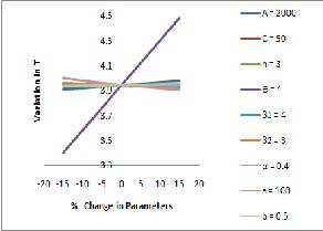
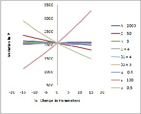
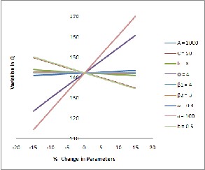
Fig 3: Relationship between optimal values and parameters

without shortages

Table 2

Sensitivity analysis of the model-without shortages

It is observed that the costs are having significant in- fluence on the cycle length, profit per unit time, Quantity. As
the ordering cost A increases, optimal cycle length 𝑇 ∗, opti- mal selling price 𝑠∗ , and optimal ordering quantity 𝑄∗ are increasing and the optimal profit 𝑃∗, is decreasing. When the cost per unit C increases, optimal selling price 𝑠∗ , and optimal profit 𝑃∗ are increasing and , optimal cycle length
𝑇 ∗, and optimal ordering quantity 𝑄∗ are decreasing. When the holding cost h increases, optimal cycle length 𝑇 ∗, optimal profit 𝑃∗, and optimal ordering quantity 𝑄∗ are decreasing and optimal selling price 𝑠 ∗, is increasing.
As the scale parameter θ increases, optimal cycle
length 𝑇 ∗, optimal selling price 𝑠∗ , optimal profit 𝑃∗, and optimal ordering quantity 𝑄∗ , are increasing. As the shape parameter 𝛽1 increases optimal cycle length 𝑇 ∗, optimal sell- ing price 𝑠∗ , optimal profit 𝑃∗, and optimal ordering quanti- ty 𝑄∗ , are decreasing. As the shape parameter 𝛽2 increases optimal cycle length 𝑇 ∗, optimal selling price 𝑠 ∗, optimal profit 𝑃∗, and optimal ordering quantity 𝑄∗ , are decreasing.
As the mixing parameter ‘𝛼’ increases optimal cycle
length 𝑇 ∗, optimal selling price 𝑠∗ , optimal profit 𝑃∗, and
optimal ordering quantity 𝑄∗ , are decreasing.
As the demand parameter ‘a’ increases optimal cycle
length 𝑇 ∗, optimal profit 𝑃∗, and optimal ordering quantity
𝑄∗ , are decreasing and optimal selling price 𝑠∗ , is increasing.
As the demand parameter ‘ b’ increases optimal selling price
𝑠∗ , optimal profit 𝑃∗, and optimal ordering quantity 𝑄∗ , are

International Journal of Scientific & Engineering Research, Volume 5, Issue 7, July-2014 262

ISSN 2229-5518

decreasing and optimal cycle length 𝑇 ∗, is increasing.

5 CONCLUSION

This paper deals with the inventory model for deteriorating items with two component mixture of Pareto distribution. Here it is assumed that the life time of the commodity is ran- dom and follows a two component mixture of Pareto distribu- tion. The two component mixture of Pareto distribution char- acterizes the heterogeneous nature of life time of the commod- ity. In many practical situations the procurement is done from different sources/vendors. For the first time, the utility of two component mixture of Pareto distribution in inventory models is done because of its close reality to the practical situations. Here it is considered that the demand is a function of selling price. The optimal pricing and ordering policies of the model are derived. The sensitivity analysis of the model reveals that the deteriorating distribution parameter and costs have signif- icant influence on the pricing and ordering policies of the model. It is also observed that this model includes the inven- tory model for deteriorating items given by Srinivasa Rao et.al [12] as a particular case for specific value of the mixing pa- rameter. By suitable estimation of the cost and deteriorating distribution of the parameters, the operational managers of market yards/ ware houses/production processes can obtain the optimal schedules using historical data. It is also possible to develop inventory model for deteriorating items with het- erogeneous life times and stock dependent demand which can be taken up elsewhere.

REFERENCES

[1] Covert, R.P. and Philip, G.C. (1973): An EOQ model for items with

Weibull distribution deterioration, AIIE. Trans 5, 323 – 326.

[2] Ghare, P.M. and Schrader, G.F (1963): A Model for exponentially

decaying inventories, Journal of Industrial Engineering, Vol.14, 238 –

243.

[3] Goyal, S.K. and Giri, B.C (2001): Recent trends in modeling of deteri-

orating inventory’, European Journal of Operational Research, Vol.

134, 1 – 16.

[4] Essey Kebede Muluneti and Srinivasa Rao. K., (2011): EPQ Models for deteriorating items with stock-dependent production rate and time- dependent demand having three parameter Weibull decay, Int. J. Operational Research, Vol. 14, No. 3, 271-300.

[5] Lakshminarayana, J., Srinivasa Rao, K. and Madhavi, N. (2005): Or-

dering and pricing of an inventory model for deteriorating items with second’s sale, Indian Journal of Mathematics and Mathematical Sciences, Vol.1, No. 2, 83-92.

[6] Liao, J. J and Huang , K. N. (2010): Deterministic inventory model for

deteriorating items with trade credit financing and capacity con-

straints , Computers & Industrial Engineering

[7] Raafat, F. (1991) : Survey of literature on continuously deteriorating

inventory models, Journal of the Operational Research Society, Vol.

42, No.1, 27-37.

[8] Sridevi, G., Nirupama Devi, K. and Srinivasa Rao. K., (2010): Inven- tory model for deteriorating items with Weibull rate of replenish- ment and selling price dependent demand, International Journal of the Operational Research, Vol. 9, No.3, 329-349.

[9] Srinivasa Rao, K., Uma Maheswara Rao, S.V. and Venkata Subbiah,

K. (2011): Production inventory models for deteriorating items with production quantity dependent demand and Weibull decay, Interna- tional Journal of the Operational Research, Vol. 11, No.1, 31-53.

[10] Srinivasa Rao. K., Sridevi, G., Nirupama Devi, K. (2010): Inventory model for deteriorating items with Weibull rate of production and demand as a function of both selling price and time, Assam Statisti- cal Review, Vol. 24, No. 1, 57-78.

[11] Srinivasa Rao. K., P.V.G.D.Prasada Reddy and Y. Gopinath (2006): Inventory model with hypo exponential life time having demand as function of selling price and time, Journal of Ultra Science for Physi- cal Sciences, Vol. 18, No.1, 87-98.

[12] Srinivasa Rao, K., Vivekananda Murthy, M. and Eswara Rao, S.

(2005): Optimal Ordering and pricing policies of an inventory models for deteriorating items with generalized Pareto life time’, Journal of Stochastic Process and its Applications, Vol.8, No.1, 59-72.

[13] UmaMaheswara Rao, S.V, Srinivasa Rao, K., and Venkata Subbiah,

K., (2011): Production Inventory Model for deteriorating items with

on hand inventory and time dependent demand, Jordan Journal of

Mechanical and Industrial Engineering, Vol.5, No. 2, 31-53.

[14] Venkata Subbiah, K., Uma Maheswara Rao, S.V., and Srinivasa Rao, K.(2010): An Inventory Model for perishable items with alternating rate of production. International Journal of Advanced Operations Management, Vol. 10, No.1, 123-129.