International Journal of Scientific & Engineering Research, Volume 4, Issue 12, December-2013 1791

ISSN 2229-5518

Inflectoin s-shaped model: Order Statistics

Dr. R. Satya Prasad1, K. Prasada Rao2 and G. Krishna Mohan3

Associate Professor, Dept. of Computer Science & Engg., Acharya Nagrjuna University Nagarjuna Nagar, Guntur, Andhrapradesh, India. profrsp@gmail.com

Professor, Dept. of MCA, CMRIT, Kundalahalli, Bangalore.

prasadarao.k@cmrit.ac.in
Reader, Dept. of Computer Science, P.B.Siddhartha college Vijayawada, Andhrapradesh, India. km_mm_2000@yahoo.com

ABSTRACT-Software Reliability is defined as the probability that the software will work without failure for a specified period of time. Software Reliability Growth Model (SRGM) is one of the most well-known theoretical models for estimating and predicting software reliability in development and maintenance. In SRGM, software reliability growth is defined by the mathematical relationship between the time span of program testing and the cumulative number of detected faults. SRGMs can estimate the total number of initial faults in the target software by applying the well-known SRGM described by non-homogeneous Poisson processes (NHPPs) to the bug data. In this paper we proposed a control mechanism based on order statistics of the cumulative quantity between observations of time domain failure data using mean value function of inflection S-shaped model, which is Non Homogenous Poisson Process (NHPP) based. The Maximum Likelihood Estimation (MLE) method is used to derive the point estimators of a two-parameter distribution.

Index terms: SRGM, NHPP, MLE, order statistics, time domain, grouping, inflection S-shaped.

IJ————S—————— E———————R———

1 INTRODUCTION

To improve and to understand the logic behind process control methods, it is necessary to give some thought to the behavior of sampling and of averages. If the length of a single failure interval is measured, it is clear that occasionally a length will be found which is towards one end of the tails of the process’s normal distribution. This occurrence, if taken on its own, may lead to the wrong conclusion that the process requires adjustment. If, on the other hand, a sample of four or five is taken, it is extremely unlikely that all four or five failure interval lengths will lie towards one extreme end of the distribution. If, therefore, we take the average or length of four or five failure intervals, we shall have a much more reliable indicator of the state of the process. Sample failure interval length or means will vary with each sample taken, but the variation will not be as great as that for single failure.
In the distribution of mean lengths from samples
of four failures, the standard deviation of the means, called the standard error of means, and denoted by the symbol SE, is half the standard deviation of the individual Time between failures taken from the process. When n=4, half the spread of the parent distribution of individual TBF. The smaller spread of the distribution of sample averages provides the basis for a useful means of detecting changes in processes. Any change in the process mean, unless it is extremely large, will be difficult to detect from individual results alone. A large number of individual readings would,
therefore, be necessary before such a change was confirmed.
Noise is inherent in the software failure data. A transformation of data is needed to smooth out the noise. Malaiya et al., (1990) tried to smooth out the noise by data grouping. They noticed that the smoothing improves quality initially as the size increases and becomes worse as the group size is large. Order statistics deals with properties and applications of ordered random variables and functions of these variables. The use of order statistics is significant when failures are frequent or inter failure time is less.

1.1 Order Statistics

Order statistics deals with properties and applications of ordered random variables and functions of these variables. The use of order statistics is significant when inter failure time is less or failures are frequent. Let A denote a continuous random variable with probability density function(pdf ), f(a) and cumulative distribution function(cdf ), F(a), and let (A1 , A2 , …, Ak) denote a random sample of size k drawn on A. The original sample observations may be unordered with respect to magnitude. A transformation is required to produce a corresponding ordered sample. Let (A(1) , A(2) , …, A(k)) denote the ordered random sample such that A(1) < A(2) < … < A(k); then (A(1), A(2), …, A(k)) are collectively known as the order statistics derived from the parent A. The various
IJSER © 2013 http://www.ijser.org

International Journal of Scientific & Engineering Research, Volume 4, Issue 12, December-2013 1792

ISSN 2229-5518

distributional characteristics can be known from
Balakrishnan and Cohen(1991).

1.2 SPC

Statistical Process Control (SPC) is about using control charts to manage software development efforts, in order to effect software process improvement. The practitioner of SPC tracks the variability of the process to be controlled. The early detection of software failures will improve the software reliability. The selection of proper SPC charts is essential to effective statistical process control implementation and use. The SPC chart selection is based on data, situation and need (MacGregor, 1995). Many factors influence the process, resulting in variability. The causes of process variability can be broadly classified into two categories, viz., assignable causes and chance causes.
The control limits can then be utilized to monitor
the failure times of components. After each failure, the time
can be plotted on the chart. If the plotted point falls between the calculated control limits, it indicates that the process is in the state of statistical control and no action is warranted. If the point falls above the UCL, it indicates that the process average, or the failure occurrence rate, may
have decreased which results in an increase in the item

Rational sub grouping of data

We have seen that a subgroup or a sample is a small set of observations on a process parameter or its output, taken together in time. The two major problems with regard to choosing a subgroup relate to its size and the frequency of sampling. The smaller the subgroup, the less opportunity there is for variation within it, but the larger the sample size the narrower the distribution of the means, and the more sensitive they become to detecting change (Oakland, 2008).
A rational subgroup is a sample of items or
measurements selected in a way that minimizes variation among the items or results in the sample, and maximizes the opportunity for detecting variation between the samples. With a rational subgroup, assignable or special causes of variation are not likely to be present, but all of the effects of the random or common causes are likely to be shown. Generally, subgroups should be selected to keep the chance for differences within the group to a minimum, and yet maximize the chance for the subgroups to differ from one another. At this stage it is clear that, in any type of
process control charting system, nothing is more important

IJSER

between failures. This is an important indication of possible
process improvement. If this happens, the management should look for possible causes for this improvement and if the causes are discovered then action should be taken to maintain them. If the plotted point falls below the LCL, It indicates that the process average, or the failure occurrence rate, may have increased which results in a decrease in the failure time. This means that process may have deteriorated and thus actions should be taken to identify and causes may be removed. It can be noted here that the whole process involves the mathematical model of the mean value function and knowledge about its parameters. If the parameters are known they can be taken as they are for the further analysis is. If the parameters are not known, they have to be estimated using a simple data by any admissible, efficient method of distribution. This is essential because
the control limits depend on mean value function which
than the careful selection of subgroups. The software failure
data is in the form of <failure number, failure time>. By grouping a fixed number of data into one, the noise values may compensate each other for that period and thus the noise inherent in the failure data is reduced significantly (Malaiya et al., 1990).

2 NHPP MODEL

The Non-Homogenous Poisson Process (NHPP) based software reliability growth models (SRGMs) are proven to be quite successful in practical software reliability engineering (Musa et al., 1987). The main issue in the NHPP model is to determine an appropriate mean value function to denote the expected number of failures experienced up to a certain time point. Model parameters can be estimated by using Maximum Likelihood Estimate (MLE).
intern depend on the parameters.
Let

{N (t ) , t ≥ 0}

denote a counting process
The control limits for the chart are defined in such a manner that the process is considered to be out of control
representing the cumulative number of faults detected by
the time ‘t’. An SRGM based on an NHPP with the mean
when the time to observe exactly one failure is less than
value function (MVF)

m (t ) is the mean value function,

LCL or greater than UCL. Our aim is to monitor the failure
process and detect any change of the intensity parameter.
When the process is in control, there is a chance for this to
representing the expected number of software failures by time ‘t’ can be formulated as (Lyu, 1996).

n

happen and it is commonly known as false alarm. The traditional false alarm probability is to set to be 0.27%

P {N (t ) = n} = m (t )

n!

e− m(t ) ,

n = 0,1, 2,...

although any other false alarm probability can be used. The

λ (t )

is the failure intensity function, which is
actual acceptable false alarm probability should in fact
depend on the actual product or process (Swapna et al.,
proportional to the residual fault content. In a more
1998).
general NHPP SRGM
IJSER © 2013 http://www.ijser.org

λ (t ) can be expressed as

International Journal of Scientific & Engineering Research, Volume 4, Issue 12, December-2013 1793

ISSN 2229-5518

λ (t ) = dm(t )

dt

b (t ) a (t ) − m (t )

. Where,

a (t ) is

3 ILLUSTRATING THE MLE METHOD.

Based on the inter failure data given in Data Set#1

the time-dependent fault content function which includes the initial and introduced faults in the program and b (t )

is the time-dependent fault detection rate. In software reliability, the initial number of faults and the fault detection rate are always unknown. The maximum likelihood technique can be used to evaluate the unknown parameters.

Inflection S-shaped model

Software reliability growth models (SRGM’s) are
useful to assess the reliability for quality management and testing-progress control of software development. They have been grouped into two classes of models concave and S-shaped. The most important thing about both models is that they have the same asymptotic behavior, i.e., the defect
& Set#2, we demonstrate the software failures process
through failure control chart. We used cumulative time between failures data for software reliability monitoring. The use of cumulative quality is a different and new

∧

approach, which is of particular advantage in reliability. ‘ a ’

∧

and ‘ b ’ are Maximum Likely hood Estimates (MLEs) of
parameters ‘a’ and ‘b’ and the values can be computed using iterative method for the given cumulative time between failures data.
The probability density function of a two- parameter inflection S-shaped model has the form:

be−bt (1 + b )

detection rate decreases as the number of defects detected
(and repaired) increases, and the total number of defects

f (t ) =

.

(1 + b e−bt )2

detected asymptotically approaches a finite value. The
inflection S-shaped model was proposed by Ohba in 1984.
The corresponding cumulative distribution function is:

(1 − e−bt )

This model assumes that the fault detection rate increases
throughout a test period. The model has a parameter, called

F (t ) =

.

1 + b e−bt

the inflection rate, which inIdicateJs the ratio oSf detectable ER

a 1 − e−bt

faults to the total number of faults in the target software.
True, sustained exponential growth cannot exist in the real

Mean Value Function of the model is m(t ) =

( )

.

1 + b e−bt

world. Eventually all exponential, amplifying processes
will uncover underlying stabilizing processes that act as
limits to growth. The shift from exponential to asymptotic
For rth order statistics, the mean value function is

r

 a 1 − e−bt 

r

growth is known as sigmoidal, or S-shaped, growth.

expressed as m (t ) = 



 .

1 + b e−bt 

Ohba models the dependency of faults by postulating the following assumptions:
• Some of the faults are not detectable before some other
faults are removed.
• The detection rate is proportional to the number of detectable faults in the program.

 

The failure intensity function of rth order is given as:

λ r (t ) = mr (t ) .

To estimate ‘a’ and ‘b’ , for a sample of n units, first obtain the likelihood function:

n

r

• Failure rate of each detectable fault is constant and
identical.

The Likelihood function L = e− m (tn )

∏

i =1

λ r (t ) .

• All faults can be removed.

Assuming [Ohba 1984b]: b (t ) = b

Take the natural logarithm on both sides, The Log
Likelihood function is given as (Pham, 2006):

n

1 + b e−bt

This model is characterized by the following mean value function:

log L

= ∑

i =1

log λ r (t ) − mr (t )

ar rbe−(bt ) (1

e−bt )r −1 (1 b )

n  i − i + 

m(t ) =

a (1 − e−bt )

= ∑ log  

(3.1)

 − + 

1 + b e−bt

where ‘b’ is the failure detection rate, and ‘ b ’ is the

i =1

(1 + b e bti )r 1

inflection factor. The failure intensity function is given as:

 =a

1 − e−(bt

n )  



abe−bt (1 + b )

−    

λ (t ) = .

 1 + b e−(bt

n )  

(1 + b e−bt )2

   

The parameter ‘a’ is estimated by taking the partial
derivative w.r.t ‘a’ and equating to ‘0’.
IJSER © 2013 http://www.ijser.org

International Journal of Scientific & Engineering Research, Volume 4, Issue 12, December-2013 1794

ISSN 2229-5518

r  1 + b e

−btn 

a = n  

(3.2)

 1 − e−(btn ) 

The parameter ‘b’ is estimated by iterative Newton

g (bn )

Raphson Method using

bn +1 = bn − , which is

g '(bn )

substituted in finding ‘a’. Where
expressed as follows.

g (b ) & g ' (b )

are
Taking the Partial derivative w.r.t ‘b’ and equating to ‘0’.

n n 

t e−(bti ) (r −1)

t e−(bti ) (r + 1) b 

i i

g (b ) = +

 −t +

(bt )

+ (bt ) 

∑ i − −

b =1

1 − e i

1 + b e i 

i  

nrt e−btn (1 + b )

(3.3)

− n

(1 − e−btn )(1 + b e−btn )

Again partially differentiating w.r.t ‘b’ and equating to 0.

 

Table 4.2: Data Set #2 [SYS 2]

' ( )

n ∑(

2 −(bti ) ) 

r −1

(r + 1) b 

g b = − 2 + −ti e b i =1

+

 (1 − e−(bt ) )2

(1 + b e

−bti 2 



 

 e−(btn ) (1 − e−(btn ) ) + e−(btn ) (1 + b e−(btn ) ) 

+ nrt 2 (1 + b )  

(3.4)

IJSER

 (1 − e−(bt ) )2 (1 + b e−bt )2 

4 TIME DOMAIN DATA SETS FOR ORDERED STATISTICS

Data Set #1, #2: The Real-time Control System Data

The data sets were listed in "DATA" directory Containing 45 industry project failure data sets in the Handbook of Software Reliability Engineering (Lyu, 1996).

Table 4.1: Data Set #1 [SYS 1]

IJSER © 2013 http://www.ijser.org

International Journal of Scientific & Engineering Research, Volume 4, Issue 12, December-2013 1795

ISSN 2229-5518

5 ESTIMATED PARAMETERS AND THEIR CONTROL

LIMITS

The estimated parameters and the calculated control limits of the Mean Value Chart for Data Set#1 to Data Set #2 with the false alarm risk, α = 0.0027 are given in Table 5.1. Using the estimated parameters and the estimated limits, we calculated the control limits UCL= m(tU ) , CL= m(tC ) and LCL= m(tL ) . They are used to find whether the software process is in control or not. The estimated values of ‘a’ and ‘b’ and their control limits for both 4th-order and 5th-order statistics are as follows.

Table 5.1: Parameter estimates and Control limits of 4 & 5

order

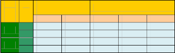
Dat Or a de Set

11

Estimated

Parameters

Control Limits

12

6 DISTRIBUTION OF TIME BETWEEN FAILURES

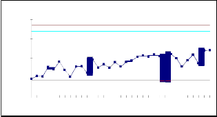
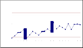
The mean value successive differences of rth order

failure control chart

IJSE10.000000 R

cumulative time between failures data of the considered

UCL 4.906847

CL

data sets are tabulated in Table 6.1 to 6.4. Considering the
mean value successive differences on y axis, failure
numbers on x axis and the control limits on Mean Value chart, we obtained figure 6.1 to 6.4. A point below the

1.000000

0.100000

0.010000

2.456738

0.006631

control limit

m(tL )

indicates an alarming signal. A point

LCL

above the control limit m(tU ) indicates better quality. If the

0.001000

1 2 3 4 5 6 7 8 9 10 11 12 13 14 15 16 17 18 19 20 21 22 23 24 25 26 27 28 29 30 31 32 33

failure number

points are falling within the control limits it indicates the software process is in stable.

Table 6.1: Successive differences of 4 order mean values of Data Set 1

Figure 6.1: 4 order Mean Value Chart for Data Set 1

Table 6.2: Successive differences of 5 order mean values

Data Set 1

IJSER © 2013 http://www.ijser.org

International Journal of Scientific & Engineering Research, Volume 4, Issue 12, December-2013 1796

ISSN 2229-5518

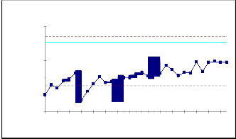
failure control chart

failure control chart

10.0000000

1.0000000

UCL CL

3.7724912

1.8887940

10.000000

1.000000

UCL CL

2.493964

1.248667

0.1000000

0.100000

0.010000

0.0100000

0.0010000

LCL

0.0050983

0.001000

0.000100

LCL

0.003370

1 2 3 4 5 6 7 8 9 10 11 12 13 14 15 16 17 18 19 20 21 22 23 24 25 26

1 3 5 7 9 11 13 15 17 19 21 23 25 27 29 31

IJSER

failure number

Figure 6.2: 5 order Mean Value Chart for Data Set 1

Table 6.3: Successive differences of 4 order mean values of Data Set 2

failure number

Figure 6.3: 4 order Mean Value Chart for Data Set 2

Table 6.4: Successive differences of 5 order mean values of Data Set 2

IJSER © 2013 http://www.ijser.org

International Journal of Scientific & Engineering Research, Volume 4, Issue 12, December-2013 1797

ISSN 2229-5518

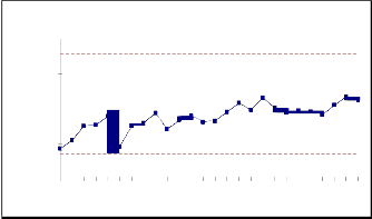
10.0000000

1.0000000

UCL CL

failure control chart

1.996139

0.9994177

Software Reliability Growth Model”. The 3rd IEEE International Symposium on High-Assurance Systems Engineering. IEEE Computer Society.

[7]. Lyu, M. R., (1996). “Handbook of Software Reliability

Engineering”. McGraw-Hill publishing, ISBN 0-07-039400-8.

[8]. Oakland. J., (2008). “Statistical Process Control”, Sixth Edition, Butterworth-Heinemann, Elsevier.

[9]. Malaiya, Y. K., Sumit sur, Karunanithi, N. and Sun, Y. (1990).

“Implementation considerations for software reliability”, 8th

Annual Software ReliabilitySymposium, June 1.

0.1000000

0.0100000

0.0010000

LCL

0.0026977

Author’s profile:
Dr. R. Satya Prasad Received Ph.D. degree in Computer Science in the faculty of Engineering in 2007 from Acharya Nagarjuna University, Andhra Pradesh.

1 2 3 4 5 6 7 8 9 10 11 12 13 14 15 16 17 18 19 20 21 22 23 24

failure number

Figure 6.4: 5 order Mean Value Chart for Data Set 2

7 CONCLUSION

The 4 and 5 order Time Between Failures are plotted through the estimated mean value function against the rth failure (i.e 4 & 5) serial order. The parameter estimation is carried out by Newton Raphson Iterative method. Data

He received gold medal from Acharya Nagarjuna University for his outstanding performance in a first rank in Masters Degree. He is currently working as
Associative Professor and H.O.D, in the Department of
Computer Science & Engineering, Acharya Nagarjuna
University. His current research is focused on Software
Engineering. He published 70 research papers in National
& International Journals.
Set#1 and Data Set#2 haveIshownJthat, some oSf the mean ER

value successive differences have gone out of calculated
control limits i.e below LCL at different instants of time. In
Data Set#1, the successive differences of mean values are within the control limits for both 4th and 5th order. In Data Set#2, the failure process is detected at an early stage for both 4th and 5th order i.e. in between UCL and LCL, which indicates a stable process control. The early detection of software failure will improve the software Reliability. Hence we conclude that our method of estimation and the control chart are giving a Positive recommendation for their use in finding out preferable control process or desirable out of control signal. When the successive differences of failures are less than LCL, it is likely that there are assignable causes leading to significant process deterioration and it should be investigated. On the other hand, when the successive differences of failures have exceeded the UCL, there are probably reasons that have lead to significant improvement.

REFERENCES

[1]. Balakrishnan. N., Clifford Cohen. A., (1991). “Order Statistics and

Inference”, Academic Press, INC. page 13.

[2]. MacGregor, J.F., Kourti, T., (1995). “Statistical process control of multivariate processes”. Control Engineering Practice Volume 3, Issue 3, 403-414.

[3]. Musa, J.D., Iannino, A., Okumoto, k., (1987). “Software Reliability: Measurement Prediction Application”. McGraw-Hill, New York.

[4]. Ohba, M., (1984). “Software reliability analysis model”. IBM J.

Res. Develop. 28. 428-443.

[5]. Pham. H., (2006). “System software reliability”, Springer.

[6]. Swapna S. Gokhale and Kishore S.Trivedi, (1998). “Log- Logistic

Mr. K.Prasad Rao, Working as a Professor, Dept. of M.C.A, CMR Institute of Technology. He is having 22 years of experience as a Head & Lecturer in Computer Science field. He Published papers in 3 National and 1 International journals. He is pursuing Ph.D at Acharya
Nagarjuna University. His research interests lies in
Software Engineering.

Mr. G. Krishna Mohan, working as a Reader in the Department of Computer Science, P.B.Siddhartha College, Vijayawada. He obtained his M.C.A degree from Acharya Nagarjuna University, M.Tech from JNTU, Kakinada, M.Phil from Madurai Kamaraj University and pursuing Ph.D from
Acharya Nagarjuna University. He qualified AP State Level Eligibility Test. His research interests lies in Data Mining and Software Engineering. He published 21 research papers in various National and International journals.
IJSER © 2013 http://www.ijser.org