is shown in figure 4.1.
4. After getting estimated values prediction error is calculated to find prediction accuracy which is given in the equation
3.2.5:
International Journal of Scientific & Engineering Research, Volume 4, Issue 12, December-2013 567
ISSN 2229-5518
Prof. Thirumahal R., Ms. Deepali A. Patil
Abstract— Missing data imputation technique means a strategy to fill missing values of a data set in order to apply standard methods which require completed data set for analysis. These techniques retain data in incomplete cases, as well as impute values of correlated variables. Most of the existing algorithms are not able to deal with a situation where particular column contains many missing values. In this paper, we present an Autoregressive model based Imputation of missing values and its improved version. ARL Impute is effective for a situation where particular column contains many missing values but it is not able to deal with situation where many columns conatins many missing values. Thus, we present an Improved ARL based imputation to estimate missing values. Data preprocessing output is given to the input of the prediction techniques namely linear prediction. This technique is used to predict the future values based on the historical values. The performance of the algorithm is measured by performance metrics like precision and recall.
Keywords- Autoregressive model (AR), Missing value estimation, Time series analysis, Linear prediction.
—————————— ——————————
Missing data imputation techniques can be used to improve data quality. Several methods have been applied in data min- ing to handle missing values in database. Data with missing values could be ignored, or a global constant could be used to
mainly on how to expedite the search if a particular time point (Column) conatins single or many missing values in sny type of dataset, less attension has been paid to the methods that exploit this search for many missing values at many time
IJSER
fill missing values (unknown, not applicable, infinity), such as
attribute mean, attribute mean of the same class, or an algo-
rithm could be applied to find missing values. K-nearest
neighbor imputation [1] can find missing values in a particular column but if many missing values are present then this method will give incorrect result. ARL [2] will perform when there are many missing values at particular time points, and
even when the experiments for time points fail or are missing. But if many columns with many missing values are present then this method is not applicable . Improved ARL works well to estimate many missing values from many columns.
The task of time-series prediction has to do with forecasting [10] future values of the time series based on its past samples. In order to do this, one needs to build a predictive model for the data. Data preprocessing output is given to the input of the prediction techniques namely linear prediction and quadratic prediction.Prediction makes use of existing variables in the database to predict unknown or future values of interest
Existing algorithms in temporal data mining has focused
————————————————
• Ms. Deepali A. Patil is currently pursuing masters degree program in computer engineering in TSEC,University of Mumbai, India, E-mail: deep.patil1987@gmail.com
• Prof. Thirumahal R. is Assistant Professor in department of Information technology in TSEC, University of Mumbai, India, Email: r_thirumahal@yahoo.com
points.
The approach proposed in paper [1] describes the KNN impute algorithm to find missing values from microarray time series dataset. The k-nearest neighbor (KNN) method selects genes with expression values similar to those genes of interest to impute missing values. The drawbacks of KNN imputation are the choice of the distance function and it searches through all the dataset looking for the most similar instances. In order to overcome this problem ARL impute was introduced.
The LLSimpute (Local Least Squares Imputation) algorithm [8] predicts the missing value using the least squares formulation for the neighborhood column and the non-missing entries. It works well but the time complexity is higher. Due to above disadvantages in [2] they discussed ARL based missing value estimation method that takes into account the dynamic prop- erty of temporal data and the local similarity structures in the data.
The approach in [2] uses autoregressive-model-based missing value estimation method (ARLS impute) which is effective for the situation where a particular time point contains many missing values or where the entire time point is missing. But this method does not estimate missing values form many col- umns. Thus, improved version of ARL was introduced
To predict the future time series vales using clustering or training the neural network [13] , however incur a very high update cost for either mining fuzzy rules or training parame- ters in different models. Therefore, they are not applicable to efficient online processing in the stream environment, which requires low prediction and training costs. To overcome this drawbacks Xiang et al [4] proposed three approaches namely
IJSER © 2013 http://www.ijser.org
International Journal of Scientific & Engineering Research, Volume 4, Issue 12, December-2013 568
ISSN 2229-5518
polynomial, Discrete Fourier Transform (DFT) and probabilis- tic, to predict the unknown values that have not arrived at the system and answer similarity queries based on the predicted data.
In this work, we describe and evaluate two methods of estima- tion for missing values in Synthetic control dataset [5]. We compare our ARL and Improved ARL based methods by cal- culating error rate using NRMSE to show the accuracy. And also we present the polynomial approach that predicts future values based on the approximated curve of the most recent values.
ARL Impute [2] and [10] is not able to deal in the situation where a many time points contain many missing values or where the entire database is missing. Improved ARL is an ef- fective method which finds the missing values for more than one columns of missing data.
Improved ARL is a modification of ARL Impute so that this
If we separate the observed data from missing data and split A
in the block matrix, the equation can be written as:
e=Bx+Cy ……………………………..3.1.3
Where B = [B1 , B2 · · · ] and C = [C1, C2 · · · ] are block sub matrices of A corresponding to the respective locations of ob- served data y and missing data x. Finally the missing data can be calculated from B# (pseudo inverse of B).The correspond- ing equation is given by:
x= -B# Cy …………………….3.1.4
Example (IMPROVED ARLI): t={1,2,3,4,5,6} ft={28.7812,31.3381,28.9207,25.3969,32.8717,36.0253}; f={28.7812,31.3381,28.9207,25.3969,0,0};
t={1,2,3,4,5,6,7}
ft1={ 34.4632, 31.2834, 33.7596, 27.7849,7.569, 29.2171,
32.337};
f1={ 34.4632, 31.2834,0,0,0, 29.2171, 32.337};
Predicted missing values in f are:
33.444517818996474 at t=5.0
IJSER
algorithm includes all the steps of ARL Impute. Improved
ARL Impute algorithm finds missing values from different
columns and therefore coefficient matrix will be calculated for
every column. Then put those coefficients into the cublic spline equation to get the predicted values.
AR coefficients [3] can find by or cubic spline interpolation method. AR model can be described in equation as follows:
37.0461820669976 at t=6.0
Predicted missing values in f1are:
28.97423999999749 at t=3.0
27.73036999999391 at t=4.0
27.746439999989708 at t=5.0
y j = Y j a j +∈ j
………………………3.1.1
Prediction technique described in paper [4] uses H historical
where, aj is the coefficient matrix., ∈ j is a sequence of inde-
pendent identically distributed normal random variable with
values (x1. . . xH ) to predict ∆t consecutive values in the fu- ture. Without loss of generality, let x1 be the value at time
mean zero. It means that any given value y j
in the time series
stamp 1, x2 at time stamp 2, and so on. In linear prediction,
is directly proportional to the pervious value Y j
plus some
this assumes that all the H+∆t values can be approximated by
random error ∈ j. As the number of AR parameters increase,
y j becomes directly related to additional past values.
Here aj coeffiecint matrix will be calculated for each column. Let us assume that (y1,y2,….ys) are the observed data and {x1,
. . . , xm} are the missing data. Estimation of missing data in
matrix form is given by:
e=Az ………………………………………………3.1.2
where z is a column vector that consists of the observed data y and the missing data x, and A is a Toeplitz matrix whose col- umn number is n and row number is n- p , which is written as:
a single line in the form of equation 3.2.1:
x=a.t + b …………………………………………………... (3.2.1)
where, t is the time stamp, x is the estimated value, and pa-
rameters a and b characterize these H+∆t data.
Algorithm of prediction technique:
Input: No. of historical values H, No. of predicted values Δt Output: Prediction of future values at timestamp t and pre- diction error
1. Specify the no. of historical values (H) and predicting values
− a p
− a1
1 0 0
(Δt).
A =
0 − a p
− a1 1
0
2. Linear prediction is defined in the equation 3.2.2:
x=a.t+b ……………………………………………….. (3.2.2)
IJSER © 2013
0 0
− a p − a1
1
International Journal of Scientific & Engineering Research, Volume 4, Issue 12, December-2013 569
ISSN 2229-5518
where, a and b are coefficients, t is timestamp and x is esti- mated value.
3. The coefficients a and b is computed using equation 3.2.3 and 3.2.4 respectively:
To calculate positive and negative values thresholds are set for number of historical values and prediction error.
a=12. ∑t =1
H
(i − (H + 1) / 2) ⋅ xi / H ( H +1)( H −1)
i / H (1− H )
…. (3.2.3)
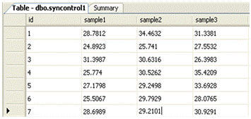
Missing values are estimated for Synthetic control chart da- taset [5] using Improved AutoRegressive (AR) Model. Dataset
b=6. ∑t =1 (i − (2H + 1) / 3) ⋅ x
….. (3.2.4)
is shown in figure 4.1.
4. After getting estimated values prediction error is calculated to find prediction accuracy which is given in the equation
3.2.5:
Errorpred
(Ti ) =
m + ∆t −1
∑ (tij
j = m
− t 'ij )2 / E
max
……………………………………………. (3.2.5)
Where, t ' ij
corresponds to the predicted value of tij . Emax is
the maximum possible error between actual and predicted series. And Errorpred (Ti ) is the relative error.
Example:
X= (34.4632, 31.2834, 33.7596, 27.7849, 27.1159, 29.2171, 32.337)
Fig 4.1. Synthetic contol chart Time series dataset
No of historical values: 4
IJSER
Enter the number of predicted values: 3
a=-1.7558700000000016 b=36.21245
Predicted next 3 values: t5.0=29.18896999999999 t6.0=27.43309999999999 t7.0=25.677229999999987
Prediction error=0.6224089545612033
Prediction techniques can be measured by two parameters namely precision and recall. To calculate Precision and Recall TP (True Positive), TN (True Negative), FP (False Positive), FN (False Negative), P (No of Positives), N (No of Negatives) val- ues are taken into account. Precision, Recall, TP rate, FP rate can be calculated by using following equation:
Precision=TP/ (TP+FP) Recall= TP/ (TP+FN)
TP, FP, TP and FN can be calculated as follows:
1. TN / True Negative: case was negative and predicted nega-
tive.
2. TP / True Positive: case was positive and predicted positive.
3. FN / False Negative: case was positive but predicted nega-
tive.
4. FP / False Positive: case was negative but predicted posi-
tive.
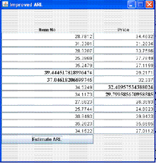
Fig 4.2. Output Of Improved ARL Impute
As shown in figure 4.2, User has to enter zero for many values in more than one column to show that the value is missing and then click on the estimate button. Here, after pressing Es- timate button message dialog box shows the predicted value which is approximately similar to original value. After estima- tion, a predicted value is imputed instead of zero. Here, the disadvantage of ARL Impute which will estimate many miss- ing values from a particular column is overcome by estimating many missing values from more than two columns.
IJSER © 2013 http://www.ijser.org
International Journal of Scientific & Engineering Research, Volume 4, Issue 12, December-2013 570
ISSN 2229-5518
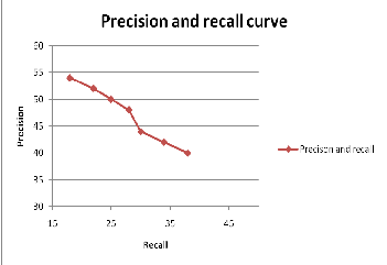
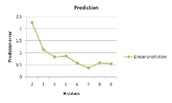
Figure 4.3 shows the performance of linear prediction by vary- ing number of Historical (H) values over prediction error. Graph shows that linear predictions have errors that first de- crease and then increase when H increases. This indicates that the most recent values have more importance in predicting future values, whereas too few historical data may result in a high prediction error. X-axis of the graph indicates number of H- values in the database and Y-axis indicates Prediction error in percentage.
Figure 4.4 Precision and recall curve
This application focuses on the task of estimating the missing values from database and imputes them again to the database so that database is completed with related values. Here the idea is to find the missing values indicated by zeros and esti- mate and impute those using different algorithms Also, the predictions of future time series values are done by using line- ar prediction. Performance of prediction depends on the preci- sion and recall curve.
Figure 4.3 Performance of Linear prediction using error prediction vs H- values
The performance of the prediction was measured by Precision- Recall curve which are shown in Figure 4.4. Based on these curves, accuracy of the proposed algorithm can be measured. Precision- Recall curve can be obtained by plotting recall in x axis and precision in y axis. Fig 4.4 shows that recall value is decreased with respect to increasing value of precision.
ARL Impute estimates many missing values form a particular column and Improved ARL Impute estimates many missing values form more than one column. Linear prediction algo- rithm predicts the future values based on the historical values.
Here, experimental results are promising: The performance of the prediction was measured by Precision-Recall curve which shows that recall value is decreased with respect to increasing value of precision.
Besides using different probabilistic algorithms many further improvements can be done. Here we are focusing only on number of missing values and number of columns but not on length of a column.
[1] Hui-Huang Hsu, Andy C. Yang, Ming-Da Lu, “KNN-DTW Based Missing Value imputation for Microarray Time Series Data”, journal of computers, vol. 6, no. 3, March 2011.
[2] Miew Keen Choong, Member, IEEE, Maurice Charbit, Member, IEEE, and Hong Yan, Fellow, IEEE “Autoregressive-Model-Based Missing Value Estimation for DNA Microarray Time Series Data”,IEEE trans- actions on information technology in biomedicine, VOL. 13, NO. 1, JANUARY 2009
[3] David Sheung Chi Fung, “Methods for the Estimation of Missing
Values in Time Series”, a thesis Submitted to the Faculty of Commu-
IJSER © 2013 http://www.ijser.org
International Journal of Scientific & Engineering Research, Volume 4, Issue 12, December-2013 571
ISSN 2229-5518
nications, Health and Science Edith Cowan University Perth, Western
Australia.
[4] Xiang Lian, Lei Chen, Efficient Similarity Search over Future Stream Time Series, IEEE Transactions On Knowledge And Data Engineer- ing, VOL. 20, NO. 1,pp- 40-55, JANUARY 2008.
[5] UCI machine learning repository, http://archive.ics.uci.edu/ml, 2010. [6] M.J. Shepperd and M.H. Cartwright, “Dealing with Missing Software
Project Data”, Empirical Software Engineering Research Group School of Design, Engineering & Computing, Bournemouth Universi- ty.
[7] Trevor Hastie, Robert Tibshirani, Gavin Sherlock, Michael Eisen, Patrick Brown, David Botstein, “Imputing Missing Data for Gene Expression Arrays”
[8] Y.Tao , D. Papadias, and X. Lian, Reverse KNN Search in Arbitrary
Dimensionality, Proc. 30th Int’l Conf. Very Large Data Bases (VLDB
’04), 2004.
[9] O. Troyanskaya, M. Cantor, G. Sherlock, et al., "Missing value estima- tion methods for DNA microarrays," Bioinformatics, vol. 17, pp. 520-
525, 2001.
[10] P. M. T. Broersen, “Finite sample criteria for autoregressive order selection,” IEEE Trans. Signal Process., vol. 48, no. 12, pp. 3550–3558, Dec 2000.
[11] S.Policker and A. Geva, “A New Algorithm for Time Series Predic- tion Temporal Fuzzy Clustering”, Proc. 15th Int’l Conf.Pattern Recognition (ICPR’00), 2000.
[12] S. Friedland, A. Niknejad, and L. Chihara, “A simultaneous recon- struction of missing data in DNA microarrays”, Linear Algebra Appl., vol. 416, pp. 8–28, 2006.
[13] S.Policker and A. Geva, “A New Algorithm for Time Series Predic- tion by Temporal Fuzzy Clustering”, Proc. 15th Int’l Conf.Pattern Recognition (ICPR ’00), 2000.
[14] Zhang, Weili Wu and Huang, Mining Dynamic InterdimensionAsso- ciation Rules for Local -scale Weather Prediction, Proceedings of the
28th Annual International Computer Software and Applications Con- ference, pp.200-204, 2004..
[15] Vilalta and S. Ma, Predicting Rare Events in TemporalDomains, Proc.
Int’l Conf. Data Mining (ICDM ’02), 2002.
[16] Abdullah Uz Tansel et al, Temporal Databases-Theory, Design and
Implementation, Benjamin/Cummings publications, 1993.
[17] E. Acuna and C. Rodriguez, “The treatment of missing values and its effect in the classifier accuracy,” Classification, Clustering and Data Mining Applications, pp.639-648, 2004.
IJSER © 2013 http://www.ijser.org