International Journal of Scientific & Engineering Research The research paper published by IJSER journal is about Implementation of MUSIC Algorithm for a Smart Antenna System for Mobile Communications 1

ISSN 2229-5518

Implementation of MUSIC Algorithm for a Smart

Antenna System for Mobile Communications

T.Nageswara Rao1, V.Srinivasa Rao2

Abstract— This paper presents practical design of a smart antenna system based on direction-of-arrival estimation and adaptive beam forming. Direction-of-arrival (DOA) estimation is based on the MUSIC algorithm for identifying the directions of the source signals incident on the sensor array comprising the smart antenna system. Adaptive beam forming is achieved using the LMS algorithm for directing the main beam towards the desired source signals and generating deep nulls in the directions of interfering signals. The smart antenna system designed involves a hardware part which provides real data measurements of the incident signals received by the sensor array. Results obtained verify the improved performance of the smart antenna system when the practical measurements of the signal environment surrounding the sensor array are used. This takes the form of sharper peaks in the MUSIC angular spectrum and deep nulls in the LMS array beam pattern.

Index Terms— Smart antennas, DOA estimation, adaptive beam forming, least mean

——————————  ——————————

1 INTRODUCTION

ireless networks face ever-changing demands on their Spectrum and infrastructure resources. Increased mi- nutes of use, capacity-intensive data applications, and
the steady growth of worldwide wireless subscribers mean carriers will have to find effective ways to accommodate in- creased wireless traffic in their networks. However, deploying new cell sites is not the most economical or efficient means of increasing capacity Smart antennas provide greater capacity and performance benefits than standard antennas because they can be used to customize and fine-tune antenna coverage pat- terns to the changing traffic or radio frequency (RF) conditions in a wireless network [1][6].A smart antenna is a digital wire- less communications antenna system that takes advantage of diversity effect at the source (transmitter), the destination (re- ceiver), or both. Diversity effect involves the transmission and/or reception of multiple RF-waves to increase data speed and reduce the error rate. In conventional wireless communica- tions, a single antenna is used at the source, and another single antenna is used at the destination. Such systems are vulnerable to problems caused by multipath effects.
Basic diagram of smart antenna is shown in Fig.1
From this which is explained about the beam forming one
represents the desired user and interfering user towards this direction antenna will focus the radiation beam forming. Max- imum radiation pattern provide towards the desired user and less beam provide the interfering user (unwanted user).
Functional Block Diagram of a smart antenna system as shown in fig 2

Fig.1. Basic diagram of smart anteena

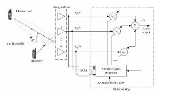
Fig.2 A functional block diagram of a smart antenna system [3].

————————————————

1. T.Nageswara rao is currently working as Assitant Professor in Department of ECE, Anurag engineering college, Andhrapradesh,India, PH-(91)9494446508.E-mail: nagu.iitkgp17@gmail.com

2. V.Srinivasa Rao is currently working as Associate professor in Depart- ment of ECE Anurag engineering college,Andhrapradesh,India, PH- (91)9440083948. E-mail: vsrao.anurag@gmail.com

The use of smart antennas can reduce or eliminate these prob- lems resulting in wider coverage and greater capacity. A smart antenna system at the base station of a cellular mobile system is depicted in Fig. 3. It consists of a uniform linear antenna array for which the current amplitudes are adjusted by a set of com- plex weights using an adaptive beam forming algorithm.
The adaptive beam forming algorithm optimizes the array output beam pattern such that maximum radiated power

http://www.ijser.org

ISSN 2229-5518

is produced in the directions of desired mobile users and deep nulls are generated in the directions of undesired signals representing co-channel interference from mobile users in adja- cent cells. Prior to adaptive beam forming, the directions of users and interferes must be obtained using a direction-of ar- rival (DOA) estimation algorithm [2]. DOA estimation as well as adaptive beam forming these models and simulations was based on pre-defined input data signals that simulate the sig-
origin. The coordinates of the mth element are noted (xm, ym, zm).
There are L incoming signals due to L sources. The signals
as they travel across the array undergo a phase shift. The phase
shift between a signal received at the reference element and the
same signal received at element m is given by

 m   m (t)  1 (t)  kxm cos sin  kym sin  sin  kzm cos

(1)
nal environment surrounding the sensor array. This paper in- vestigates the performance of smart antenna algorithms using

Where

k  2



is the propagation constant in free space for

an experimental setup that involves a hardware part used to
collect real data measurements of the received signals imping-

linear array of equispaced elements with element spacing

ing on the smart antenna sensor array In this way, a more rea-

x  d

aligned along the x-axis such that the first element is

listic and accurate description of the signal environment sur- rounding the sensor array is used to provide the input for the MUSIC algorithm being investigated.

situated at the origin, we have xm=(m-1)d and ym=zm=0.as we

suppose that the signals are coming in horizontally we also have

   /2 .

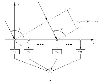
 m  kd (m 1) cos

(2)

Note that 1=0. Let’s define the incoming signal at the array element 1 due to the lth sourve by

( ) ( ) j 2 f0t

sl t

 ml t e

(3)

Where ml(t) is the modulating function of the lth source and f0 the frequency of the carrier signal. The incoming signal at ele- ment m will be in that case

x (t)  m (t)e j (2 f0t  m )  n

(t)  s (t)a

()  n

(t)

Fig.3 Uniform linear arreay with M elements

The paper is discussed as follows: Section 1 Introduc-

m l m l m m

Where
(4)
tion Section 2 develops the theory of smart antenna systems. Section 3 Signal Model and its MATLAB Implementation, Section 4 presents performance results for the designed smart

am (l )

 e j m

 e j kd ( m1) cosl

(5)

antenna system. Finally, conclusions are given in Section 5.
.

2. THEORETICAL MODEL FOR AN ANTENNA ARRAY

Intelligent antenna definition

An”intelligent” antenna is an array of spatially separated
and where nm(t) is a random noise component on the mth ele- ment, which includes background noise and electronic noise generated in the mth channel. It is assumed to be temporally white with zero mean and variance equal to .
We can now define the steering vector as

 1 

 

 a2 ( l ) 

antennas whose outputs are fed into a weighting network. The
part that makes the antenna array ”intelligent” is the signal



a(l )   a

.... 

 

processing unit which calculates the weights that produce the desired radiation pattern of the array.

2.1 Conventional Charging

An antenna array can be arranged in any arbitrary fashion, but

 m ( l ) 

(6)

in this paper we will limit ourselves to linear arrays with un- iformly spaced sensors (see figure 3). Let M be the number of antenna elements [4][5]. Usually an array has a reference ele- ment. Let’s suppose that this reference element is located at the
Now if we consider all sources simultaneously, the signal at
the mth element will be

http://www.ijser.org

ISSN 2229-5518

L L where I is an identity matrix of dimensions M and S (L

x  m (t)e j ( 2 f0t  m )  n

(t) 

s (t)a

( ) n

(t)

by L matrix) denotes the source correlation

m  l m

l 1



l 1

l m l m

(7)

3. SIGNAL MODEL AND ITS MATLAB

Let’s define the array signal vector by

IMPLEMENTATION

We know that for a real antenna, vector x represents the signals

X (t)  (x1 (t)x2 (t)x3 (t)........xm (t)........xM (t))

the incoming signal vector by

(8)

received at the different antenna elements

The signal vector:

We have seen in the previous section

S (t)  (s (t)s (t)s (t)........s (t)........s (t ))T

the noise vector by

(9)

R  ASAH

and

  2 I

(18)

n(t)  (n (t)n (t)n (t)........n (t)........n (t ))T

(10)

X (t)  As(t)  n(t)

(19)

and the steering matrix (dimensions M by L) by

A  (a(1 )a(2 )a(3 )........a(l )........a(L ))

(11)

Where s represents the incoming signal vector where each ele- ment represents the signal sent by one User. One of these sig- nals is modeled by

( ) ( ) j 2 f0t

We can now write in matrix notation

sl t

 ml t e

(20)

X (t)  As(t)  n(t)

Let’s denote the weights of the beam former as

W  (w w w ........w ........w )T

(12)

(13)

Where ml(t) denotes the complex modulating function. The structure of the modulating function reflects the particular modulation used in the system.

3.1 The MUSIC Algorithm

DoA Estimation Methods

We have seen that for some beam formers, but also for
where w is called the array weight vector. The total array out- put will be

other applications, it can be useful to gather information about the users’ positions. Methods which extract this information from the incoming signals are called Direction of Arrival (DoA) Estimation Methods.

y(t) 



m1

w m xm

 W H X (t )

(14)

There are mainly two categories of such methods. The
methods of the first one are called Spectral Estimation Me-
thods. They include the MVDR (Minimum Variance Distor-
sionless Response) Estimator, Linear prediction method, MEM
Where superscripts T and H, respectively, denote the trans-
pose and complex conjugate transpose of a vector or matrix. If
the components of x (t) can be modeled as zero mean statio-
nary processes, then for a given w, the mean output power of
the process is given by

P  E[ y(t) y* (t)]  W H R W

xx (15)

where E[·] denotes the expectation operator and Rxx is the ar- ray correlation matrix defined by
(Maximum Entropy Method), MLM (Maximum Likelihood Method). The second category is formed by the Eigen structure Methods.
They include the MUSIC (Multiple Signal Classification) algo-
rithm, the Min-Norm Method, the CLOSEST Method, the ES-
PRIT (Estimation of Signal Parameters via Rotational Inva-
riance Technique) algorithm, and others. There are some more
methods that do not fit in any of these two categories.

3.2 Mathematical background of MUSIC

Computation of the correlation matrix The MUSIC algorithm

Rxx

 E[ X (t) X H (t)]

(16)

requires the correlation matrix Rxx. In practice however, the exact value of
Algebraic manipulation leads to
Rxx = E[x(t)xH(t)] ( 21)

R  ASAH

  2 I

(17)

is not available. Instead we have to replace Rxx with it’s esti- mate. An estimate of Rxx using N samples x(n), n = 0, 1,

http://www.ijser.org

ISSN 2229-5518

2,…......N − 1 of the array signals may be obtained using a sim- ple averaging scheme



spectrum are guaranteed to correspond to the true angle of arrival of the signals incident on the array.

Some peaks in the MUSIC spectrum P (  ) are usually very

N 1

Rxx   X [n]X N n0

H [n]

(22)

high, so that it is more convenient to plot the log of the MUSIC
spectrum. The positions of these peaks are then determined by looking for the zero crossings of the derivate of log (P(Ø)).
Note that in order to make the MUSIC algorithm work, the
incident signals mustn’t be correlated.
Where x (n) denotes the array signal sample, also known as the array snapshot, at the nth instant of time, with t replaced by nT and the sampling time T omitted for the ease of notation. For simplicity of notation, the estimate of Rxx is called Rxx too.

Eigenvalue decomposition of the correlation matrix

Next we have to do an eigenvalue decomposition of Rxx. Rxx is of dimension M by M, so it has generally M eigenvalues. Denoting the M eigenvalues of Rxx in descending order by λm, m = 1,…,..,M and their corresponding unit-norm eigenvectors by Um, the matrix takes the following form:

R    H

xx (23)

with the diagonal matrix

MATLAB implementation

Important preliminary remark: In all the subsequent MATLAB

simulations, the direction of a source is parameterized by the vari- able  (theta) and not by the variable  . In this paper we ob- served both Static Cases and Dynamic case

4 SIMULATION RESULTS

4.1 Static Case

Let’s consider a simple case where M is 5 and L is 3. Signal to noise ratio (SNR) is 20 dB. The step size for calculating the MUSIC spectrum is 0.01 and the number of snapshots N is 10. Figure 4 shows from top to bottom the spectrum P, log (P) and it’s derivate.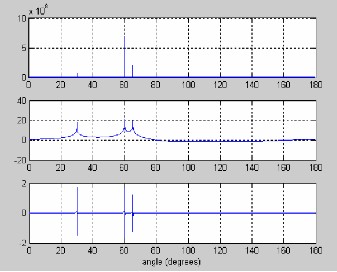

 1 0 0 

 

  . m . 

 0 0

M 

  (24)

containing the eigenvalues in it’s diagonal and

 (U1....U1....UM )

3.3 The MUSIC spectrum

The MUSIC spectrum is defined as

(25)

P( ) 

Where

aH ( ) H a( )

(26)

Figure 4 Spectrum P, log (P) and its derivative which id represented as linear scale

N  (UL1.....UM )

is the collection of the noise eigenvectors and a( ) The

(27)

figure 4 represents the user positions P i.e. user one,
user two, user three, represents the MUSIC spectrum of
the signals (three user signals) (log (P)) and represents the
zero crossing (its derivative) As you can see, the peaks in P
are very high

matrix

  N

is a projection matrix onto the noise subspace.

INFLUENCE OF SIGNAL TO NOISE RATIO

For steering vectors that are orthogonal to the noise subspace, the

denominator of (26) will become very small, and thus peaks will occur in P(  ) corresponding to the angle of arrival of the signal. When the ensemble average of the array input covariance matrix is known and the noise can be considered uncorrelated and identi- cally distributed between the elements, the peaks of the MUSIC

In this section, we analyze the influence of the SNR. Fig 5 is taken from the previous section (SNR = 20 dB and N = 10). We know from the previous section that this situation gives very good results for the positions.

http://www.ijser.org

ISSN 2229-5518

Dynamic case:

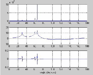
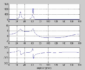
Fig: 5 results for SNR=20dB and N=10

Fig: 6 results for SNR=10dB and N=10

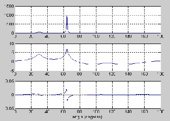
Fig: 7 results for SNR=0dB and N=10

Let’s now have a look at the simulations for the dynamic case. This time we have M = 9 and L = 5and the main user is moving from position 50°to position 90° The window size is 10 samples. SNR is 20 dB. The spectrum step size is 0.1 and not
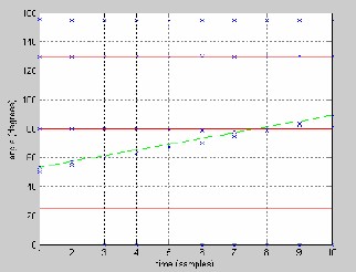
0.01 in order to make the simulation faster. We now consider a first example where the user moves from 50° to 90° in 1000 samples which means that we have 100 windows with 10 sam- ples. This corresponds to a speed of 0.04 deg/sample. The re- sult is shown in Fig.8 Of course; at the moment when the mov- ing user is crossing the user at 80° the algorithm will only detect 4 users, because the two crossing users mask each other. Let’s now consider a second example where the user moves from 50° to 90°in 100 samples. This means that we only have 10 windows with 10 samples.
This corresponds to a speed of 0.4 deg/sample, so the user moves by 4 degrees during one window. As you can see in Fig.
9, the results are much more imprecise this time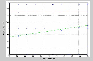

Fig 8: Real user positions and calculated user positions for user speed of 0.04 deg/sample.

Fig.9 Real user positions and calculated user positions for user speed of 0.4 deg/sample in linear scale

http://www.ijser.org

ISSN 2229-5518

5 CONCLUSION

Referring to the paper, one can say that the goals have been largely reached. A direction of arrival algorithm (MUSIC) has been implemented in MATLAB, followed by a parametric study of the static case. After that, a possible solution for the dynamic case has been proposed a detailed treatment of vari- ous methods of estimating the DOA’s has been provided by including the description, limitation, and capability of each method and their performance comparison as well as their sen- sitivity to parameter perturbations. This paper provides refer- ences to studies where array beam-forming and DOA schemes are considered for mobile communications systems.

REFERENCES

[1] L.C. Godara, "Applications of Antenna Arrays to Mobile Communications.I.

Performance Improvement, Feasibility, and System Considera- tions,"Proceedings of IEEE, Volume 85, Issue 7, Pages1031-1060, July

1997.

[2] L.C. Godara, "Application of Antenna Arrays to Mobile Communications.II.

Beamforming and Direction-of-Arrival Considerations,"Proceedings of

IEEE, Volume 85, Issue 8, , Pages1195-1245. August 1997

[3]

―A Setup for the Evaluation of MUSIC and LMSAlgorithms for a

Smart Antenna System‖ Journal of Communications, vol. 2, no. 4, June

2007‖

[4] Nuteson, T.W.; Mitchell, G.S.; Clark, J.S.; Haque, D.S. ―Smart antenna systems for wireless applications‖ ; Antennas and Propagation Society In- ternational Symposium, 2004. IEEE Volume 3, 20-25 Page(s):2804 - 2807

Vol.3 June 2004

[5] Bellofiore, S.; Balanis, C.A.; Foutz, J.; Spanias, A.S.; ―Smart-antenna sys- tems for mobile communication etworks. Part 1. Overview and antenna de- sign‖ Volume 44, Issue 3, Page(s):145 – 154 Jun 2002

[6] A. J. Paulraj, D. Gesbert, C. Papadias Paulraj, gesbert, papadias, ―Smart Antennas for Mobile Communications in encyclopedia for electrical engi- neering‖, john wiley publishing co. 2000.

http://www.ijser.org