International Journal of Scientific & Engineering Research, Volume 6, Issue 1, January-2015 739

ISSN 2229-5518

Hydrodynamic Analysis of a Column Structure of a Petroleum Storage Tank

Inegiyemiema Morrision and Nitonye Samson

Abstract— Column structures are used extensively in the Niger Delta Area of Nigeria to position drilling platforms and petroleum storage facilities in the offshore environment. To avoid failure of the structures it is necessary to carry out hydrodynamics analysis of the columns in order for them to withstand environmental forces of wind, wave and current. The designed column will be subjected to other different forms of load such as the dead weight and light weight besides the environmental loads, but the project focuses only on the environmental loads in which environmental data will be obtained from agencies and applied into Morrision’s equation to analyse and obtain the von misses stress, tensile stress and compressive sress. The results obtained are verified by carring out software analysis using ansys. The accepted result is subjected to API Code to ensure that it fails within an allowable limit.

Index Terms— Current, Dead weight, Enviromental forces, Misses stress, Piles, Wave and W ind

——————————  ——————————

1 INTRODUCTION

HE loading condition of this concrete structure will be divided into two categories, known as life loads and dead loads. The dynamic effect that comes out as a result of this type of loading will also be considered. These will in-
clude the dead, live, environmental and dynamic loads
Dead loads are the weights of the storage tank and any permanent equipment and appurtenant structure which do not change with the mode operation. Therefore dead load will include:
• Weight of the storage facility in air, including
where appropriate the weight of the concrete column.
• Weight of equipment such as appurtenant structures permanently mounted on the storage facility.
Life loads are the loads imposed on the structure during its use and which may change either during a mode of opera- tion or from one mode of operation to another [5]
1 The weight of consumable supplies and liquids in storage
tank.
Environmental loads are loads imposed on the storage tank
by natural phenomenon including wind, wave current,
earthquake etc. In this particular case, we are going to only consider wind, current and wave. This is because the pro- ject will be sited in an intermediate water depth of about twenty five point three meters and is not within an earth

————————————————

• Inegeyemiema Morrison, Department of Marine Engineering, Rivers State University of Science and Technology, Port Harcourt, Rivers State Nigeria. E-mail: ineng22002@yahoo.com

• Nitonye Samson, Department of Marine Engineering, Rivers State Uni- versity of Science and Technology, Port Harcourt, Rivers State Nigeria. E-

mail: nitonyes@yahoo.com
quake prone region.
These are loads imposed on the storage tank due to re-
sponse to an excitation of a cyclic nature or due to reacting
impact to impact. Excitation of the structure may be caused by waves, wind or machinery. Impact may be caused by a barge or a boat berthing against the platform or by drilling operations.

1.1 Loading Conditions

Design environmental load conditions can be referred to as those forces imposed on the storage tank structure by the selected design event: whereas, operating environmental load conditions are those forces imposed on the structure by a lesser event which is not severe enough to restrict normal operations.

1.2Design Loading Conditions:

The Storage tank will be designed for appropriate loading conditions which will result or produce the most severe effects on the structure. The loading conditions should be a combination of environmental conditions and appropriate dead and live loads in the following manner:
• The first condition will be the operating environmental conditions combined with dead loads and maximum live loads appropriate to normal operations of the storage tank
• Secondly the operating environmental conditions combined with dead loads and minimum live loads appropriate to normal operations of the storage tank.
• Thirdly, the design environmental conditions with dead loads and maximum live loads appropriate for combining with extreme conditions.

IJSER © 2015 http://www.ijser.org

International Journal of Scientific & Engineering Research, Volume 6, Issue 1, January-2015 740

ISSN 2229-5518

• Fourthly, the design environmental conditions with dead loads and minimum live loads appropriate for combining with extreme conditions.
Hydrostatic forces acting on the structure below the water line including external pressure and buoyancy is my main focus on this project.
The fixed storage facility will be situated in an intermediate water depth; therefore the loads can be represented by their static equivalents. That means the static analysis is ade- quate enough to describe the true dynamic loads induced by the structure [2].
The steps and method employed in calculation of determin- istic static design wave forces on a fixed storage tank. We assume that there is no dynamic response and there is no distortion of the incident wave by the storage facility. The procedure for a given wave directions begins with the spec- ification of the design wave height and associated wave period, storm water depth and current profile. The proce- dure for the calculation of the wave force follows these steps.
• An apparent wave period is determined which accounts for the Doppler effect of the current on the wave.
• The two-dimensional wave kinematics will be determined from an appropriate wave theory for the specified wave height, storm water depth and apparent period.
• The horizontal components of wave-induced particle velocities and accelerations will be reduced by the wave kinematics factor, which accounts primarily for wave directional spreading.
• The effective local current profile is determined by multiplying the specified current profile by the current blockage factor.
• The effective local current profile is combined vectorially with the wave kinematics to determine locally incident fluid velocities and accelerations for use in Morrison’s equation.
• Member dimensions are increased to account for marine growth.
• Drag and inertia force coefficients are determined as functions of wave and current parameters and member shape, roughness (marine growth), size and orientation.
• Wave force coefficients for the conductor array are reduced by the conductor shielding factor.
• Local wave/current forces are calculated for all storage tank members using the Morrison’s equation.
• The global force is computed as the vector sum of all the local forces.

1.3 Current

The current load can be described as the vector sum of the tidal, circulation, and storm generated currents. The off- shore location varies with the relative magnitude of these compounds and thus their importance for computing loads. Current Profile: Is to determine the variation of current speed and direction with depth.
Current Force only: where current is acting alone (ie no waves). The drag force according to the API specification will be determined by this equation dU/dt = 0
Current Associated with Waves: There can be possible su- perposition of the current and waves. Where this superpo- sition happens it is necessary the current velocity should be added vectorialy to the wave particle velocity before the total force is computed [3].

2 Materials and Methods

The appropriate wave theory that was chosen is the Line-
ar/Airy wave theory. This is because the dimensionless wave steepness and the dimensionless relative depth of the parameters on an ATKINS graph fall on the intermediate water depth. We assume that the fluid layer has a uniform mean depth, and that the fluid flow is inviscid, incompress- ible and irrotational. The simpliest and most applied wave theory is the linear wave theory. It is also called small am- plitude wave theory. The wave has the form of a sine curve and the free surface profile is written in the followin simple form η = a Sin(Kx-ωt).

2.1 Finite Water Depth

The designed fixed offshore storage facility operates in an intermediate water depth. The following equations will be required to calculate the wave loading on the offshore structure [7] [10].
Note: ω = 2π/T, k = 2π/λ,
is the wave number, λ is the wave length , T = wave period
, Ϛa = wave amplitude, g = acceleration due to gravity, t =
time, x = direction of wave propagation z = vertical coordi-
nate, d = water depth, total pressure in the fluid = pd – ρgz
+ po, po = atmospheric pressure

IJSER © 2015 http://www.ijser.org

International Journal of Scientific & Engineering Research, Volume 6, Issue 1, January-2015 741

ISSN 2229-5518

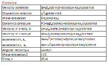
Velocity Potentials

𝜙 = 𝑔 𝜁𝑎 𝑐𝑐𝑐 ℎ 𝑘(𝑧 +𝑑 ) cos⁡(𝜔𝜔 − 𝑘𝑘) (1)

𝜔𝑐𝑐𝑐 ℎ 𝑘𝑑

Table 2: Hydrodynamic Coefficient
Depression Relation

𝜔 2

𝑔

= 𝑘𝜔𝑎𝑘ℎ 𝑘𝑑 (2)
Table 3: Steel Properties

Wave Length 𝜆 = 𝑔𝑇


𝜔𝑎𝑘ℎ 2𝜋 𝑑 (3)

2𝜋 𝜆

Wave elevation 𝜁 = 𝜁𝑎 sig⁡(𝜔𝜔 − 𝑘𝑘) (4)
Dynamic Pressure

𝑃 = 𝜌𝑔 𝜁𝑎 cosa 𝑘 (𝑧 +𝑑 )

cosa 𝑘𝑑

sig⁡(𝜔𝜔 − 𝑘𝑘) (5)

2.3 Column Data and Material Properties:

The structure is analysed based on the given column pa- rameters from the table below.
Velocity in x – direction

𝑐𝑐𝑐 ℎ 𝑘 (𝑧 +𝑑 )

Table 4: Column Geometric characteristics
𝑢 = 𝜔𝜁𝑎

𝑐𝑠𝑘 ℎ 𝑘𝑑

sig⁡(𝜔𝜔 − 𝑘𝑘) (6)

Height 30m

Length spacing 20m
Velocity in z – direction

𝑐𝑠𝑘 ℎ 𝑘 (𝑧 +𝑑 )

Width spacing 20m
Submerge Height (d) 25.3m
𝑤 = 𝜔𝜁𝑎

𝑐𝑠𝑘 ℎ 𝑘𝑑

cos⁡(𝜔𝜔 − 𝑘𝑘) (7)
Diameter (D) 2m
Thickness (t) 0.0m
Acceleration in x-axis

𝑐𝑐𝑐 ℎ 𝑘 (𝑧 +𝑑 )

2.4 Material Properties

𝑎𝑘 = 𝜔2 𝜁𝑎

𝑐𝑠𝑘 ℎ 𝑘𝑑

cos⁡(𝜔𝜔 − 𝑘𝑘) (8)

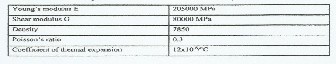
All materials specified in this report are of structural steel pipe of Group Class C ASTM Grade 50 A618 (Young’s
Acceleration in z-axis

𝑎 = −𝜔2 𝜁 𝑐𝑠𝑘 ℎ 𝑘 (𝑧 +𝑑 )

𝑐𝑠𝑘 ℎ 𝑘𝑑

sig⁡(𝜔𝜔 − 𝑘𝑘) (9)
Modulus 210MPa, Poisons’ Ratio of 0.3, Min. Yield Strength
of and Min. Tensile Strength of) [6][8].

2.5 Derived Parameter

The following parameters were derived from the linear wave theory for a finite water depth and are used as input

2.2 Environmental Data

For inplace analysis, the design storm environment shall be
100years directional independent metocean criteria. The
operating environment shall be 1 year directional
independent metocean criteria. Tables 1, 2 and 3 below
in evaluating the fluid kinematics as well as input for the fluid loading on the structure in the ansys software.

Table 5: Derived parameters to be used

Parameter Formula Values Unit

summaries the design criteria [1].
Wave Amplitude
(ζa )
H/2 3 m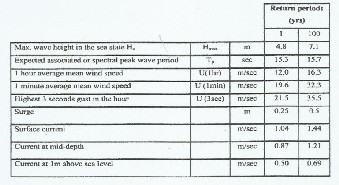

Table1: Environmental Data
Wave Frequency (ω) 0.838 Rad/secs
Wave number (K) ω2/g tanh (kd) 0.0748 m-1
N.B this is obtained from iteration process. See table

2.6 Fluid Particle Kinematics: Velocity and

Acceleration of Wave particles

• The fluid particle velocity and acceleration were determined using the linear wave theory for a fi- nite water depth shown in table 3. In this report the wave is assumed to approach the structure at an angle assumed to be zero, therefore wave direction

IJSER © 2015 http://www.ijser.org

International Journal of Scientific & Engineering Research, Volume 6, Issue 1, January-2015 742

ISSN 2229-5518

is considered uniform with the direction of the cur-
rent.
• The calculated wave velocity along the x-axis is then combined with the current’s velocity to give the total velocity, UT .
• The approach assumed there is no interaction be-
tween members in close proximity and problem is
set up within the frame work of Global axis sys- tem.

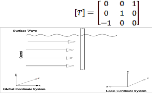
T r an s f orm at i on

The following transformation matrices were used;
• Vertical members
through the length of the members/element. All force calcu- lation was performed in the Micro soft spread sheet. See Appendix A for loads generated [5].

2.8 A Hand Calculation of Morrison’s Equation

A sample hand calculation of Morrison’s equation is done below for water depth -3 for column number one. This is done to show case the calculation procedure used and to verify the results obtained from the use of the excel spread sheet [2].

𝜔 2 = 𝑘𝜔𝑎𝑘ℎ 𝑘𝑑

𝑔

𝑢 = 𝜔𝜁𝑎

𝑐𝑐𝑐 ℎ 𝑘 (𝑧 +𝑑 )

𝑐𝑠𝑘 ℎ 𝑘𝑑

sig⁡(𝜔𝜔 − 𝑘𝑘)
After substitution
𝑢 = −1.55 f/s
𝑢 𝜔𝑐𝜔𝑎𝑡 = 𝑢 𝑤𝑎𝑤𝑤 + 𝑢 𝑐𝑢𝑐𝑐𝑤𝑘𝜔
𝑢 𝜔𝑐𝜔𝑎𝑡 = −1.5585 + 16.3 = 14.7415𝑚/𝑐
𝑎𝑘 = 𝜔2 𝜁𝑎

𝑐𝑐𝑐 ℎ 𝑘 (𝑧 +𝑑 )

𝑐𝑠𝑘 ℎ 𝑘𝑑

cos⁡(𝜔𝜔 − 𝑘𝑘)
Fig 1: Current direction [4].

2.7 Fluid loading; Morison’s equation

The hydrodynamic load acting on the structure was esti- mated according to the Morison’s equation. The Applica-
After substitution
𝑎𝑘 = 1.213f/s²
To find the in-line force at column depth -3m we apply the
Morrison’s equation
tion of this equation is based on the assumption that the
𝑓′𝑦
�

� = 1 𝜌𝐶 𝐷|𝑊 | �
𝑤′
� + 𝜌 𝜋 𝐷2 𝐶
� 𝑤′̇ �
ratio of member diameter to wave length (D/λ) is less than
0.05. The equation is as given below;

(10)
𝑓′𝑧 2
𝑓′𝑦
�𝑓′ � =

1

𝑘 𝑤′

0

4 𝑚

𝑤̇ ′

3.14q 22 0

Where
q1.05q1025q2q14.74 �

2 14.74

� + 1.2q1025

4

�1.213�
(N/m)
� 0 � = � 0
� + � 0
�(N/m)
(N/m)
The drag and inertia force are calculated using
238519.05
233834.25
4684.8

(11)
and (12)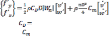

Therefore the component of force on a member in the local axis system is calculated using
(13)
Where Drag coefficient=1.05
= Inertia Coefficient=1.2
With each of this forces evaluated at 3m interval spanning

3 Results and Discussion

3.1 The Use of Excel Spread Sheet to Generate the

Forces

The forces due to the incident wave and the prevailing cur- rent at different depths on the four columns are determined using an excel spread sheet.
All the results obtained from the spread sheet are used in a
CFD method to determine the diameter of the column that will be large enough to withstand the stress and forces due to the incident wave and the current. A preliminary column diameter of two meter was first used.

IJSER © 2015 http://www.ijser.org

International Journal of Scientific & Engineering Research, Volume 6, Issue 1, January-2015 743

ISSN 2229-5518

Table 6: Hydrodynamic formulae to be imputed into the excel program

Table 8 The use of MATLAB to obtain the Constant K1

:

Table 9: Excel program to generate the environmental forces acting on pillar 1

IJSER © 2015 http://www.ijser.org

International Journal of Scientific & Engineering Research, Volume 6, Issue 1, January-2015

ISSN 2229-5518

744

VERTICAL MEME8ER1

Xi(m] Yi(m] Zi(m] xc=xicoso Coshk(z-HI Sinhk(z-HI Si nhkd Cos(wt-kxc Sin(wt-kxc U w ax az Uc=U+C

-10 -10 0 -10.0000 3.3979 3.2474 3.2474 0.6806 -0.7327 -1.9267 1.7105 1.4994 1.5426 14.3733

-10 -10 -3 -10.0000 2.74&5 2.5602 3.2474 0.6806 -0.7327 -1.5585 1.34&5 1.2129 1.2161 14.7415

-10 -10 -6 -10.0000 2.2383 2.0025 3.2474 0.6806 -0.7327 -1.2692 1.0548 0.9&n 0.9513 15.0308

-10 -10 -9 -10.0000 1.8415 1.5463 3.2474 0.6806 -0.7327 -1.0442 0.8145 0.8126 0.7345 15.2558

-10 -10 -12 -10.0000 1.5379 1.1684 3.2474 0.6806 -0.7327 -0.8720 0.6155 0.6787 0.5550 15.4280

-10 -10 -15 -10.0000 1.3U3 0.8497 3.2474 0.6806 -0.7327 -0.7441 0.4476 0.5791 0.4036 15.5559

-10 -10 -18 -10.0000 1.1531 0.5741 3.2474 0.6806 -0.7327 -0.6538 0.3024 0.5088 0.2727 15.6462

-10 -10 -21 -10.0000 1.0523 0.3275 3.2474 0.6806 -0.7327 -0.5966 0.1725 0.4643 0.1556 15.7034

-10 -10 -24 -10.0000 1.0047 0.0975 3.2474 0.6806 -0.7327 -0.5697 0.0513 0.4434 0.0463 15.7303

-10 -10 -25.3 -10.0000 1.0000 0.0000 3.2474 0.6806 -0.7327 -0.5670 0.0000 0.4413 0.0000 15.7330

Zi(m] u,=Uctosa vg=ucsi nc w, tig=axcosa vg=axsina Yig ul VL wl til vL Yil

angle between the local and global axes

Transpose Matrix

2557530 0.00 0.00

Table 10: Excel program to generate the environmental forces acting on pillar 2

IJSER ©2015 http /fwww lfser orq

International Journal of Scientific & Engineering Research, Volume 6, Issue 1, January-2015

ISSN 2229-5518

745

VERTICALMEMEBER2

Xi(m) Yi(m) Z(im) xc=xicosc Coshk(ztd Sinhk(ztd Sinhkd Cos(wt-kxc Sin(wt-kxc) U w ax az Uc=Ut(

10 -10 0 10.0000 3.3979 3.2474 3.2474 -0.6806 -0.7327 -1.9267 -1.7105 -1.4994 1.5426 14.3733

10 -10 -3 10.0000 2.7485 2.5602 3.2474 -0.6806 -0.7327 -1.5585 -1.3485 -1.2129 1.2161 14.7415

10 -10 -6 10.0000 2.2383 2.0025 3.2474 -0.6806 -0.7327 -1.2692 -1.0548 -0.9877 0.9513 15.0308

10 -10 -9 10.0000 1.8415 1.5463 3.2474 -0.6806 -0.7327 -1.0442 -0.8145 -0.8126 0.7345 15.2558

10 -10 -12 10.0000 1.5379 1.1684 3.2474 -0.6806 -0.7327 -o.8no -0.6155 -0.6787 0.5550 15.4280

10 -10 -15 10.0000 1.3123 0.8497 3.2474 -0.6806 -0.7327 -0.7441 -0.4476 -0.5791 0.4036 15.5559

10 -10 -18 10.0000 1.1531 0.5741 3.2474 -0.6806 -0.7327 -0.6538 -0.3024 -0.5088 0.2727 15.6462

Z(im) u1=Uc«JSa vg=ucsni c w, ug=axcosa vg=axsina Yig ul VL wl uL vL Yil

angle between the localandglobalaxes Transformation matrix TransposeMatrix

wn=(VL1

1DpDW %CMpnD Fdy Fdz Fiy Fiz Fx' Fy' Fz' Fx Fy Fz

twl

0 14.37 15469.28 3864.16 0.00 -222344.8 0.00 5794.00 0.00 0.00 -216550.8 216551 0.00 0.00

-3 14.74 15865.58 3864.16 0.00 -233882.9 0.00 4686.68 0.00 0.00 -229196.2 229196 0.00 0.00

-6 15.03 16176.92 3864.16 0.00 -243152.4 0.00 3816.n 0.00 0.00 -239335.7 239336 0.00 0.00

-9 15.26 16419.09 3864.16 0.00 -250486.8 0.00 3140.07 0.00 0.00 -247346.7 247347 0.00 0.00

-12 15.43 16604.34 3864.16 0.00 -256171.0 0.00 2622.45 0.00 0.00 -253548.5 253549 0.00 0.00

-15 15.56 16742.05 3864.16 0.00 -260438.0 0.00 2237.64 0.00 0.00 -258200.3 258200 0.00 0.00

SUMMATION OF FORCES 2498577 0.00 0.00

Table 11: Excel program to generate the environmental forces acting on pillar 3

IJSER ©2015 http /fwww lfser orq

International Journal of Scientific & E ngineering Resear ch, Volume 6, Issue 1, Janua ry-2015

ISSN 2229-5518

746

V miCAl ME\1fBm3

Xi(m) Yi(m) li(m) xc=xitol() Coshk(z!dJSin hk(z!dJ Sinlld Cos(wt-kxcJ Sin(wt-kxc U w ix a; U,=UtC

1CI 10 o 1o.ocro 3.3979 3.2474 3.2474 ·O.ffi06 ·0.7327 -1. 267 ·1.71(6 ·1.4994 1.5416 14.3733

10 10 ·3 10.ocro 2.7485 2.5602 12474 ·O.ffi06 ·0.732 -1.5585 ·U485 ·1.2129 11151 14.7415

angle betweente lot'al and global axes Transformation matrix Transpose Matr

wn=(Vl1iw11 l\CDpDW Y.CMpnD fdy Fdz F Fiz Fx' Fy' fz' fx Fy Fz

0 14.37 15469.18 3864.16 0.00 ·212345 0.00 5794.00 0.00 0.00 ·216550.8 216551 0.00 0.(0

·l 14.74 15865.58 3864.16 0.00 ·213883 0.00 4686.63 0.00 0.00 ·lll196.2 229196 0.00 o.w

·6 15.03 16176. 2 3864.16 0.00 ·243152 0.00 3316.n 0.00 0.00 ·239335.7 239336 0.00 o.w

- 15.26 16419.($ 3864.16 0.00 ·250487 0.00 3140.07 0.00 0.00 ·247346.7 247347 0.00 o.w

·11 15.43 1&504.J4 3864.16 0.00 ·256171 0.00 2622.45 0.00 0.00 ·253548.5 253549 0.00 O.W

·15 15.56 16742.C5 3864.16 0.00 ·260438 0.00 2237.64 0.00 0.00 ·258200.3 258200 0.00 o.w

·18 15.65 16839.ll 3864.16 0.00 ·263469 0.00 1966.17 0.00 0.00 ·261503.3 261503 0.00 0.(0

·21 15.70 16900.73 3864.16 0.00 ·265398 0.00 1794.27 0.00 0.00 ·263603.8 263604 0.00 o.w

·24 15.73 16929.73 3864.16 0.00 ·266310 0.00 1713.25 0.00 0.00 ·264596.3 264596 0.00 o.w

·25.l 15.73 16932.62 3864.16 0.00 ·266401 0.00 1705.16 0.00 0.00 ·264695.4 264695 0.00 o.w

SUMWATION OFFORCES W8577 0.00 O.W

IJSER © 2015 http /fwww lfser orq

International Journal of Scientific & E ngineering Resear ch, Volume 6, Issue 1, Janua ry-2015

ISSN 2229-5518

Table 12: Excel program to generate the environmental forces acting on pillar 4

VERTICAL MEMEBER4

Xi(ml Yi(ml Zi(ml xc=xicoSJJ Coshk(z+d Sinhk(z+dl Sinhkd Cos(wt·kxcl Sin(wt·kxc U w ax az Uc=lHC

·10 10 0 ·10.0COO 3.3979 3.2474 3.2474 0.6806 ·0.7327 -1.9267 1.7105 1.4994 1.5426 14.3733

·10 10 ·3 ·10.0COO 2.7485 2.5602 3.2474 0.6806 ·0.7327 ·1.5585 1.3485 1.2129 1.2161 14.7415

·10 10 ·6 ·10.0COO 2.2383 2.0025 3.2474 0.6806 ·0.7327 -1.2692 1.0548 o.98n 0.9513 15.0308

·10 10 ·9 ·IO.OCOO 1.8415 1.5463 3.2474 0.6806 ·0.7327 -1.0442 0.8145 0.8126 0.7345 15.2558

·10 10 ·12 ·10.0COO 1.5379 1.1684 3.2474 0.6806 ·0.7327 ·0.8720 0.6155 0.6787 0.5550 15.4280

·10 10 ·15 ·10.0COO 1.3123 0.8497 3.2474 0.6806 ·0.7327 .(),7441 0.4476 0.5791 0.4036 15.5559

747

=UfOSQ

1

vg:ucsino w1 ug=axcosa ¥g=axsina vig ul Vl wl uL vL vil

angle between the local and global axes Tra nsformation matrix

IJSER ©2015 http /fwww lfser orq

International Journal of Scientific & Engineering Research, Volume 6, Issue 1, January-2015 748

ISSN 2229-5518

3.2 Shear Force

All forces acting on each member of the structure were summed to obtain the Shear force about the baseline of the structure

Table 13: Shear Force acting on the baseline of every pile
proach. This is to create key points that will establish the nodes of the different columns of the tank. These nodes are
spaced 3m apart from each other and they form elements. The hydrodynamic forces act on these elements.
Table 14: tables specifying the modelling nodes for each col- umn

Members FX (N) FY

(N)

FZ

(N)

Vertical memeber1 2557530 0.00 0.00
Vertical memeber2 2498577 0.00 0.00
Vertical memeber3 2498577 0.00 0.00
Vertical memeber4 2557530 0.00 0.00
Total force 10112214 0.00 0

3.3 Software Simulation of the Structural Response to the Wave and Tidal Forces of the Columns

FEA is an analytical method based on approximate solutions to solve any complex engineering problem by subdividing the problems into smaller, more manageable elements.

Post-processing stage:

This involves the visualisation and the analysing of the re- sults obtained which is then used to understand the struc- tural mechanism.
From Appendix A the element type used in modelling the columns is BEAM4 (3-D Elastic Beam) which has a uniaxial element with tension, compression, torsion, and bending capabilities. The element has six degrees of freedom at each node: translations in the nodal x, y, and z directions and ro- tations about the nodal x, y, and z axes. Stress stiffening and large deflection capabilities are included (ANSYSInc, 2007) The modelling strategy employed is the bottom up ap-

Node x y z

1 0 0 0
5 0 0 -3
9 0 0 -6
13 0 0 -9
17 0 0 -12
21 0 0 -15
25 0 0 -18
29 0 0 -21
33 0 0 -24

37 0 0 -25.3

IJSER © 2015 http://www.ijser.org

International Journal of Scientific & Engineering Research, Volume 6, Issue 1, January-2015 749

ISSN 2229-5518

3.4 Boundary Conditions

Boundary Restraints: The bases of all the columns were re-

strained from moving in all the directions.

Applied Loads

Submerged parts of the columns which is twenty five point three meters are divided into 10 numbers of divisions for each vertical column. Loads were generated and applied based on these divisions at an interval of 3m except for the last division which is 1.3m interval. All loads were applied on the elements at different nodes as incident wave and cur- rent forces are added together vectorially. An axial load due the weight of the tank and the weight of the life load (petro- leum product) was applied at the top of the columns. The value of the axial force on each column is 9107114N (see Ap- pendix B). The forces act on the elements of the columns, and large deformations were not considered because it is a linear analysis.

Solution

The pre-processing and post-processing phases of the finite element method are interactive through the solution phase. The governing equations are assembled into matrix form and are solved numerically. The analysis method depends on the element type of the model, material properties and boundary conditions.
Menu Paths
Main Menu>Solution>Solve>Current LS

Post Processing

When once the solution of the model has been done then, a post processing of the model takes place. This is the reading and plotting of the results obtained from Ansys and also comparing the nodal and element von misses stresses, in- cluding their displacements. A graph of the von misses stress values are plotted against the distances of their nodes apart.

Failure criterion used: The failure prediction of the column model will be by the assessment of the von misses stress. The von misses stress is compared to the column yield stress and the ultimate strength given by the manufacturers of the steel column. The von misses stress failure criterion was cho- sen because it puts all the principal stresses into account to give an equivalent stress for more accurate prediction.

The principal stresses are
σ₁ = axial stress
σ₂ = hoop stress σ₃ = radial stress
Von misses stress, σ = (1/√2) √ [(σ₁ - σ₂)² + (σ₂ - σ₃)² + (σ₃ -
σ₁)²]

Nodal Solution

ANSYS calculates the nodal solution for each node. There- fore, the arrangement of the nodes is important to get better accuracy. The nodal Von misses stresses are compared to the element von misses stress (As shown in Appendix C). Minimum nodal von misses stress is 136568 Mpa Maximum nodal von misses stress is 0.567E+08Mpa

The Element Solution

Every element has its own stress region, because ANSYS calculates the element solution which is an average stress of the element. The element von misses stresses are the same as the nodal stresses (See Appendix D) Minimum element von misses stress is 136568 Pa
Maximum element von misses stress is 0.567E+08 Pa

3.6 Interpretation of the Deformed Shape of the Pipe

Line

The columns were displaced 0.082605m at the top but the bottom side remained stable to the sea bed. This is because the bases of the columns are firmly fixed to the sea bed and the top sides of the columns are exposed to the highest hy- drodynamic forces. As shown in Appendix E). Summary of the results obtained from FEA
The following results are obtained from the FE Analysis
from the response of the structure due to hydrody-
namic loading and axial loading;

Table 15: Summary of Obtained results

Maximum Von misses stress 0.567E+08 Pa Maximum Displacement 0.082605m Maximum Tensile stress 0.29013E+07 Pa Maximum Compressive stress -0.20608E+03 Pa Maximum bending stress 0.843E+08 Pa

3.5 Presentation of result

Validation of Result

Design Code Check

IJSER © 2015 http://www.ijser.org

International Journal of Scientific & Engineering Research, Volume 6, Issue 1, January-2015 750

ISSN 2229-5518

Design Specification

The following design code was used to check against the integrity of the storage tank columns.
• API RP 2A 21st Edition, 1993-Recommended Practice

Table 16 Result comparison

Prediction Finite Element

Method

Design Code- Allowable

for Planning Design and Constructing Fixed Off-
Axial Tension 2.9 N/mm2 207N/mm2
shore Platform-Working Stress Design.
Axial Compres-
sion
0.000206 N/mm2 4207N/mm2
The columns structural response predicted using FEM is strength checked against the above mentioned design codes using the following;

Axial Tension

•
Where
• Allowable Axial Compression
For D/t
API sec 3.2.2 a
i.e. 2/1
= Where k = constant =1
L = length of column
R = Radius of gyration
and
Since
Therefore the option below is used


Allowable Bending Stress

For
Use


• Allowable Shear Stress
API sec 3.3.4-a


• Allowable Von Mises
The results obtained from the design code shows that the allowable axial tensile, Compressive, bending and Von mises stress are 207N/mm2, 209N/mm2, 228.67N/mm2 and
276N/mm2 respectively [9].
Bending 84.3 N/mm2 247.26N/mm2
Von mises 56.7 N/mm2 276N/mm2

3.7 Overall Presentation of the Report

The highest stress concentration occur at the base of the columns. This is inline with bending moment and shear force theory of a cantilever. Therefore in the actual design of the columns the base section of the columns should be reinforced to withstand the stress and the be

Wind

Proper analysis of wind data can be used to determine the wind criteria for the design of the storage system. As with wave load, wind loads are dynamic in nature, but some structure will respond to them in nearly static fashion. For conventional fixed steel structures in relatively shallow wa- ter the contribution of wind to global loads is typically less than 10%. Sustained wind velocities will be used to compute global platform wind loads and gust velocities will be used for the design of individual structural elements.

Wind Properties.

There is variation of wind speed and direction in space and time. On length scales typical of even large offshore struc- tures, statistical wind properties (e.g. mean and standard deviation of velocity) taken over durations of the order of an hour do not vary horizontally, but is said to change with ele- vation (profile factor). Within long durations there will be shorter durations with higher mean speeds (gust factor), this means that a wind speed value is meaningful if qualified by its elevation and duration.

Wind Velocity and Force Relationship

From the API specification, the wind force on an object should be calculated by using the appropriate method such as:
F = (w/2g)(V2)Cs A
Where:
F = wind force
W=weight density of air
g = gravitational acceleration
V = wind speed
Cs = shape coefficient
A = area of object
The recommended shape coefficient Cs for a perpendicular
wind to the storage tank is 0.5
Therefore Force =10.4/(2x9.81)x16²x0.5x2x3.14x12.954x12.192

IJSER © 2015 http://www.ijser.org

International Journal of Scientific & Engineering Research, Volume 6, Issue 1, January-2015 751

ISSN 2229-5518

WIND FORCE= 67294.99N

4 Conclusions

The objective of this project is to accurately predict the re- sponse of cylindrical columns under hydrodynamic wave forces and current using the finite element method.
The type of analysis employed to achieve this objective is the linear analysis. This analysis means that due to the applied hydrodynamic forces on the columns, a resultant defor- mation of the column is seen which is directly proportional to all the inputs such as the applied loads, F, stiffness, K from material properties, geometry, and restraints. Thus, X=F/K, such that if the load is doubled, the deformation is doubled. If stiffness is doubled, the deformation is halved.
The columns were restrained at the base in all directions. It was assumed that the columns are firmly fixed to the sea bed and the foundations of the sea bed are strong and immova- ble. This means the application of hydrodynamic forces due to the waves and currents on the columns will not cause the columns to move at the base in any direction.
We assume that the deflection of the material under load is
small and linear.
The stiffness of the column material is determined by the material properties and the geometry of the column. The material properties required to simulate this kind of column analysis is divided into two parts.
Input properties are properties required to calculate a re-
sponse by the material. The properties are Young’s Modulus and Poison ratio
Failure properties are properties needed to interpret the re- sponse. They are Yield strength and the ultimate strength
The material properties employed are the ones given above under the section column data and material properties.

5 References

[1] Aluyii Baba, (2010) Fatigue Analysis of fixed jacket
offshore Structure, Masters of Science Dissertation
Newcastle University, United Kingdom.
[2] Argema (1992). Design guide for offshore struc-
tures. Paris, Technip.
[3] Atkins. W., (1991). Breaking wave loads on im-
mersed members of offshore structures. London:
HMSO American petroleum institute (API)
[4] Chakrabarti. S., (1994). Hydrodynamics of Offshore
structures. London: Computational mechanics pub-
lications Southampton.
[5] Downine Martin (2009), Lecture Note on Marine Fliud Dynamics, Newcastle University, United Kingdom.
[6] Ellenberger, J. P. (2005) Piping Systems & Pipeline

ASME CODE SIMPLIFIED. USA: McGraw-Hill

Companies, Inc.
[7] Institute, A. P. (1993) Recommended Practice for Plan-

ning, Designing and Constructing Fixed Offshore Plat- forms - Working stress Design. Washington, DC: American Petroleum Institute.

[8] Micheal F., (2002).Facility piping systems handbook.
2nd ed. U.S.A. :Mc Graw-Hill
[9] Tomlinson, M. J. (1987). Pile design and construc- tion. London, Palladian Publications Limited.
[10] Veritas, D. N. (1974) Rules for the Design, Construction and Inspection of Fixed Offshore Structures. Norway: Det Norske Veritas.

IJSER © 2015 http://www.ijser.org

International Journal of Scientific & Engineering Research, Volume 6, Issue 1, January-2015 752

ISSN 2229-5518

COLUMN SHAPE AND SECTION PROPERTIES GENER- ATED FROM ANSYS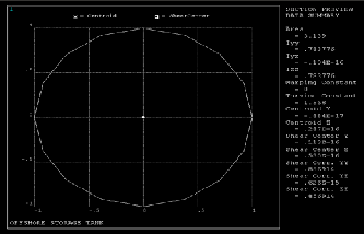

Appendix A
Appendix B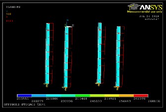

Axial load, lateral hydrodynamic pressures and maximum constraints at the base of the columns

Appendix C: Nodal Solution
Appendix D: Element Solution


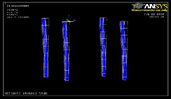
Appendix E: Displacement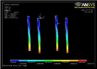

IJSER © 2015 http://www.ijser.org