the maximum and minimum limits of the generators. If there are N units, the
International Journal of Scientific & Engineering Research, Volume 5, Issue 3, March-2014 75
ISSN 2229-5518
Leelaprasad.T, N.Vijaya Anand, CH.Padmanabha Raju
Abstract— The Optimal Power Flow (OPF) plays an important role in power system operation and control due to depleting energy resources, and increasing power generation cost and ever growing demand for electric energy. As the size of the power system increases, load may be varying. The generators should share the total demand plus losses among themselves. The sharing should be based on the fuel cost of the total generation with respect to some security constraints. Conventional optimization methods that make use of derivatives and gradients are, in general, not able to locate or identify the global optimum. Heuristic algorithms such as genetic algorithms (GA) and evolutionary programming and PSO have been proposed for solving the OPF problem. Recently, a new evolutionary computation technique, called Adaptive Particle Swarm Optimization (APSO), has been proposed and introd uced. In this paper, a novel Adaptive PSO based approach is presented to solve Optimal Power Flow problem to satisfy objectives such as minimizing generation fuel cost and transmission line losses. A hybrid OPF is proposed by combining the positive aspects of Interior point method and APSO.The proposed algorithms are tested on IEEE 30 bus system using MATLAB.
Index Terms— Adaptive particle swarm optimization, Interior point method, Newton’s raphson method, Optimal power flow, Particle swarm optimization.
—————————— ——————————
HE Optimal Power Flow problem can be traced back as early as 1920’s when economic distribution of generation was the only concern. The economic operation of power
system was achieved by dividing loads among available gen- erator units such that their incremental generation costs are identical. The basic mission of a power system is to provide consumers with continuous, reliable and cost-efficient electri- cal energy. In order to achieve this aim, the system operators need for regularly adjustments of various controls such as generation outputs, transformer tap ratios, etc., to assure the continuous economic and secure system operations. This is a complex task that needs to depend highly on optimal power flow (OPF) function at power system control centers. The OPF problem optimize a selected objective function such as fuel cost via most favorable adjustment of the power system con- trol variables while on the other side satisfying the various constraints such as the equality and inequality constraints. Different types of optimization techniques have been applied in solving the OPF problems [1-18] they are nonlinear pro- gramming [1-6], quadratic programming [7-8], linear pro- gramming [9-11], Newton based techniques [12-13],
————————————————
• Leelaprasad.T,M.Tech Student, Department of EEE,Prasad V. Potluri Siddhartha Institute of Technol- ogy,Vijayawada, Andhra Pradesh, India
E-mail:leelaprasad1150@gmail.com.
• N.Vijaya Anada ,Associate Professor, Department of EEE,Prasad V. Potluri Siddhartha Institute of Technol- ogy,Vijayawada, AndhraPradesh,India.
E-mail: nidumoluvijayAnand @gmail.com
• Dr.Ch.Padmanabha Raju, Professor, Department of
EEE, Prasad V. Potluri Siddhartha Institute of Tech- nology, Vijayawada, AndhraPradesh, India.
E- mail:pnraju78@yahoo.com
sequential unconstrained minimization technique [14], and interior point methods [15-16]. The primary Interior Point (IP) is defined by the Frisch in 1955, which is a logarithmic barrier method that was later on broadly studied by Fiacco and McCormick to solve it into the nonlinearly inequality constrained problem in 1960. In 1979 Khachiyan presented an ellipsoid method that would solve a Linear Programing (LP) problem in polynomial moment. After 1984, several variants of Karmarkar’s Interior Point (IP) method have been proposed and implemented. Recently, the research in OPF such as interior point (IP) using new optimization techniques, has been obtaining a better attention in power system operation [20-21].
Heuristic algorithms, such as Genetic Algorithms (GA) [17] and evolutionary programming [18], have been recently proposed for solving the OPF problem.The results reported were promising and encouraging for further re- search in this direction. Unfortunately, recent research has identified some deficiencies in GA performance [19]. This degradation in efficiency is apparent in applications with highly epistatic objective functions, i.e. where the parameters being optimized are highly correlated. In addition, the prem- ature convergence of GA degrades its performance and re- duces its search capability.Recently, a new evolutionary computation technique, called Particle Swarm Optimization (PSO), has been proposed and introduced [22-25]. This technique combines social psychology principles in socio cognition human agents and evolutionary computations. PSO has been motivated by the behavior of organisms such as fish schooling and bird flocking. Generally, PSO is charac- terized as simple in concept, easy to implement, and compu- tationally efficient. Unlike the other heuristic techniques, PSO has a flexible and well-balanced mechanism to enhance and adapt to the global and local exploration abilities.
In this paper, a novel PSO based Hybrid approach is pro posed to solve OPF problem. The problem is formulated as an
IJSER © 2014 http://www.ijser.org
International Journal of Scientific & Engineering Research, Volume 5, Issue 3, March-2014 76
ISSN 2229-5518
optimization problem with mild constraints. In this study, the
objective functions are generation fuel cost and line losses.The proposed approach has been tested on IEEE 30-bus system.
ng is the number of generators including the slack bus
P is the generated active power at bus i
i
The economic optimal operation of power systems, con- sidering transmission constraints and supplying load demand, requires to minimize two objective functions (total generation fuel cost and active power losses) while satisfying several equality and inequality constraints. The standard OPF prob- lem can be formulated as a constrained optimization problem
a b c are the unit cost coefficients for ith generator.
Active and reactive power loss occurs in transmission lines depending on the power to be transmitted. The active
power loss equation for the k th line between buses i and j can
be given as in eqn. (4)
as follows:
min L ( x ) = P
= G (V 2 + V 2 − 2V V
cos (δ −δ ))
(4)
Subject:
Objective = min j ( x, u )
g ( x, u ) = 0, Equality constraints
Where
th
i − j j i j i j i j
Gij is i line conductance
h ( x, u ) ≤ 0, Inequality constraints
Bij
is ith line susceptance
th
Where x is the vector of dependent variable consisting of bus power P , load bus voltagesV , generator reactive power
Vi is voltage magnitude of i bus
δ is phase angle of ith bus
G1 L i
outputs QG , and transmission line loadings S1 . Hence x can be expressed as
X T = P ,V , Q ...Q , S ...S (1)
G1 L1 G1 GNG 11 1NL
Where NG and NL are number of generators, and number of transmission lines respectively.
U is the vector of independent variables consisting of genera-
The OPF problem has two categories of constraints:
The equality constraints g(x) are the real and reactive power balance equations, expressed as follows:
N
tor voltagesVG , generator real power outputs PG , except at the slack bus P , transformer tap settings T, and shunt VAR
1
P − P
i i
= Vi ∑V j ( gij cos δij + bij sin δij )
j =1
(5)
compensations QC . Hence, u can be expressed as
T
N
Qg − Qd = Vi ∑V j
j =1
( gij
sin δij + bij cos
δij )
(6)
u = VG1 ...VGNG , PG2 ...PGNG ,T1...TNT , QC1 ...QCNC (2)
Where NT and NC are the number of the regulating trans- formers and shunt compensators, respectively.
P , Q
i i
P , Q
i i
are the active and reactive power generation at bus i;
are the real and reactive power demand at bus i, V j
g and h are the load flow and operating constraints of the sys- tem respectively.
is the voltage magnitude at bus j, respectively; δij is the phase
angle difference between buses i and j, gij and bij
are the real
The most commonly used objective in the OPF problem formulation is the minimization of total fuel cost of real power generation. The individual cost of each generating unit is as- sumed to be function of active power generation and is repre- sented by quadratic curve of second order. The objective func- tion of entire power system can then be written as the sum of the quadratic cost model of each generator as given in eqn. (3)
ng
and imaginary part of the admittance (Yij ) and N is the total
number of buses.
The inequality constraints h(x, u) reflect the security limits, which include the following constraints as mentioned below:
Generator constraints
Upper and lower limits on the active power generations:
min c ( x ) = min
a P2 + bP + c
(3)
min max
∑
i =1
i gi
i gi i
P ≤ P ≤ P
i i i
i=1, 2…..NG (7)
Where, i=1, 2, 3……. ng and
Upper and lower limits on the reactive power generations:
min max
Q ≤ Q ≤ Q
i i i
i=1, 2….NG (8)
IJSER © 2014 http://www.ijser.org
International Journal of Scientific & Engineering Research, Volume 5, Issue 3, March-2014 77
ISSN 2229-5518
Upper and lower limits on the generator bus voltage magni- tude:
min max
vious velocity of the particle on its current one, coefficient
c1 and c2 are the acceleration parameters which are common-
V ≤ V ≤ V
i i i
i=1, 2….NG (9)
-ly set to 2 [28], and the parameters
r1i
and
r2i
are random
Transformer constraints:
Transformer tap settings are bounded as follows:
min max
numbers uniformly distributed in the interval [0, 1]. The value of each component in every velocity vector can be clamped to the range [- vmax, vmax] to prevent the particles leaving the
Ti ≤ Ti ≤ Ti
i=1, 2….NT (10)
search space. By the same token, the value of each component
Shunt VAR constraints
Shunt VAR compensations are restricted by their limits as fol-
lows:
min max
in every position vector can be limited to the range [xmin,
xmax].
Q ≤ Q ≤ Q
i i i
.
i=1, 2….NC (11)
PSO is a population based stochastic optimization tech- nique introduced by Kennedy and Eberhart. Like many bio- logical inspired algorithms PSO also have natural motivation like bird flocking and fish schooling. PSO is initialized with a group of random particles (solutions) and then searches for optima by updating generations. In every iteration each parti- cle is updated by following two "best" values. The first one is the best solution (fitness) it has achieved so far, this value is called Pbest. Another "best" value that is tracked by the Parti- cle swarm optimizer is the best value, obtained so far by any particle in the population; this best value is a global best and called Gbest. When a particle takes part of the population as its topological neighbors, the best value is a Pbest [26]. The number of parameters of the objective function is assumed to be n, and then the search space will be n-dimensional. The ith particle has an n-dimensional position Vector
T
In this paper the solution to OPF using PSO algorithm is
introduced, not only to minimize the generation fuel cost but
also transmission line loss. Its implementation consists of the
following six steps:
Step 1: Specify the number of generating units as the dimen-
sion. The particles are randomly generated between
the maximum and minimum limits of the generators. If there are N units, the ![]() particle is represented as fol- lows:
particle is represented as fol- lows:
( Pi = Pi , Pi , Pi ...Pi ) .
1 2 3 N
Step 2: The particles velocities are generated randomly in the range of vmin , vmax .
The maximum velocity limit is set at 10-20 % of the
dynamic range of the variables on each dimension [29,
30].
Step 3: Objective function values of the particles are evaluated
X i = ( X i1 , X i 2 ,...X in )
and an n-dimensional velocity vec-
T
using eqn. (3).These determined values are set as Pbest value of the particles.
tor Vi = (Vi1 , Vi 2 ,... Vin )
where i is a positive integer index
Step 4: The best value among all the Pbest values is identified
of the particle in the swarm. The historical best position en-
and denoted as Gbest.
countered by the
T
ith
particle is denoted
Step 5: New velocities for all the dimensions in each particle
are calculated using eqn. (12). Then the position of
as Pi = ( Pi1 , Pi 2 ,... Pin )
.Let g denote the index of the particle
each particle is updated using eqn. (13).
Step 6: The objective function values are calculated for the up-
that attained the best previous position among all the individ-
uals of the swarm, and then the global best position can be
T
dated positions of the particles. If the new value is bet- ter than the previous Pbest, the new value is set to
denoted as Pg = ( Pg1 , Pg 2 ,... Pgn )
.The fitness, value of![]()
Pbest, if the stopping criteria are met, the positions of particles represented by Gbest are the optimal solution,
particle can be calculated by f ( xi ) ,where f is the objective
function. In the process of executing PSO algorithm, a swarm is initialized by random at first, and then the global best posi- tion may be updated during the each iteration. In each of the
and otherwise the procedure is repeated from step 4.
The basic eqns of PSO (14), (15) and (16) can be con-
iterations, the position and the velocity of ith
particle are up-
sidered as a kind of difference equation.
dated with eqns. (12) and (13) as follows [27] until the iteration
termination is satisfied
k +1 k
( k ) ( k )
Vi ( k + 1) = wVi ( k ) + c1r1i ( k ) ( Pi ( k ) − X i ( k )) + c2 r2i ( k ) ( Pg ( k ) − X i ( k ))
(12)
vi = wvi
+ c1rand1 ∗
pbesti − si
+ c2 rand2 ∗
gbest − si
(14)
X i ( k + 1) = X i (k ) + Vi ( k + 1)
(13)
In the above equations, k denotes the iteration counter, w is called the inertia weigh which controls the impact of the pre-
IJSER © 2014 http://www.ijser.org
International Journal of Scientific & Engineering Research, Volume 5, Issue 3, March-2014 78
ISSN 2229-5518
The new parameters are set to each agent. The weighting coefficients are calculated as follows:
w = w
( wmax − wmin )
− ∗ iter
(15)![]()
C = 2 , C
![]()
= 2 − C
(19)![]()
max
(iter )
2 P 1 P 2
k +1
k k +1
max
1 2
The search trajectory of PSO can be controlled by the pa-
si = si
+ vi
(16)
rameters (P1, P2). Concretely, when the value is enlarged
Therefore, the system dynamics, that is, the search procedure,
can be analyzed using Eigen values of the difference equation.
Actually, using a simplified state equation of PSO, Clerc and
more than 0.5, the agent may move close to the position of
Pbest/Gbest.
Kennedy developed CFA of PSO by Eigen values [28, 29]. The velocity can be expressed as follows instead of eqns. (14) and![]()
{c1 ( pbest − x ) + c2 ( gbest − x )}
w = gbest − 2
+ x
(15):
k +1 k
( k ) (
k )
(20)
Namely, the velocity of the improved PSO can be ex-
vi = K vi
+ c1 ∗ rand1 ∗
pbesti − si
+ c2 ∗ rand2
gbest − si
pressed as follows:
(17)
k +1
( k ) ( k )
![]()
K = 2 ,
vi = wi + c1rand1 ∗
pbesti − si
+ c2 rand2 ∗
gbest − si
(21)
2 − ϕ− ϕ2 − 4ϕ
where ϕ = c1 + c2 , ϕ > 4
Where φ and K are coefficients.
(18)
The improved PSO can be expressed as follows (steps 1 and
5 are the same as PSO):
Generation of initial searching points: Basic procedures
are the same as PSO. In addition, the parameters (P1,
P2) of each agent are set to 0.5 or higher. Then, each agent may move close to the position of (Pbest, Gbest) at the following iteration.
The following points are improved to the original PSO with
Inertia Weight Approach (IWA).
The search trajectory of PSO can be controlled by in-
troducing the new parameters (P1, P2) based on the
probability to move close to the position (Pbest,
Gbest) at the following iteration.
Evaluation of searching points: The procedure is the same as PSO. In addition, when the agent becomes Gbest, it is perturbed. The parameters (P1, P2) of the agent are adjusted to 0.5 or lower so that the agent may move away from the position of (Pbest, Gbest).
The
wvk
term of (14) is modified as (17). Using the
Modification of searching points: The current searching
equation, the center of the range of particle move- ments can be equal to Gbest.
When the agent becomes Gbest, it is perturbed. The new parameters (P1, P2) of the agent may move away from the position of (Pbest, Gbest).
When the agent is moved beyond the boundary of feasible regions, Pbests and Gbest cannot be modified.
When the agent is moved beyond the boundary of feasible regions, the new parameters (P1, P2) of the agent are adjusted so that the agent may move close to the position of (Pbest, Gbest).
When the agent is moved beyond the boundary of feasible regions, Pbests and Gbest cannot be modified.
When the agent is moved beyond the boundary of feasible regions, the new parameters (P1, P2) of the agent are adjusted
So that the agent may move close to the position of
(Pbest, Gbest).
points are modified using the state eqns. (21) and (17) of
adaptive PSO.
The implementation steps of the proposed hybrid method combining IPM with APSO based algorithm can be written as follows:
Step1: Input the system data for load flow analysis
Step2: Run the power flow
Step3a: Basically the hybrid method involves two steps.
Step3b: The first step employs IPM to solve OPF
approximated as a continuous problem and intro-
duced into the initial populations of APSO.
Step3c: The second part uses APSO to obtain the final optimal
solution.
Step4: In initial population, all individuals (obtained from
IPM) are produced randomly. The main
IJSER © 2014 http://www.ijser.org
International Journal of Scientific & Engineering Research, Volume 5, Issue 3, March-2014 79
ISSN 2229-5518
reason for using IPM is that it is often closer to optimal solutions than other random individuals.
Step5: For each individual in this method, run power flow to determine generator active and reactive power outputs, shunt VAR compensators, load bus voltages, angles, tap settings can be calculated.
Step6: Evaluate the objective function values and the corresponding fitness values for each individual
Step7: Find the generation local best xlocal and global best xglobal and store them
Step8: Increase the generation counter Gen = Gen+1
Step9: Apply the APSO operators to generate new k Individ -
uals
Step10: For each new individual in this method, run power
flow to determine the generator active and reactive
power outputs, shunt VAR compensators, load bus
voltages, angles, tap settings can be calculated.
Step11: Evaluate the objective function values and the correspond-
ing fitness values for each new individual
Step12: Update the generation local best xlocal and global best
xglobal and store them
Step13: If one of stopping criterion have not been met repeat
steps 5-12. Else go to step14
Step14: Print the results.
The proposed hybrid algorithms for solving OPF prob- lem are tested on standard IEEE-30 bus system using MATLAB software and results are tabulated.
The IEEE-30 bus system consists of 30 buses, out of which six are Generator buses. The network has total active power load of 283.4 MW and reactive power load of 126.2
MVAR. Totally there are 19 control variables which consist of six Generator Bus voltages, four Tap changing transformers and nine Shunt compensators.
The PSO parameters used for simulation are summa- rized in Table-I
Here we have considered two objective functions, Objec- tive function-1 is the Cost Minimization and Objective func- tion-2 is the Loss Minimization.
Table II presents the optimal setting of the control varia- bles with objective function 1. It is observed that minimum cost was obtained using APSO-IPM method when compared
TABLE II
OPTIMAL SETTINGS OF CONTROL VARIABLES WITH GENERATION FUEL COST MINIMIZATION
TABLE – I
OPTIMAL PARAMETER SETTING FOR PSO
The proposed hybrid PSO algorithm were applied to find the optimal scheduling of the power system for the base case loading condition to minimize specified objective functions.
with other two Hybrid methods.
Table III presents the optimal setting of the control var-
iables with objective function 2. It is observed that minimum
loss value was obtained using APSO-IPM method when com-
pared with other two Hybrid methods.
Fig 1-4 shows the variation of control variables with
fuel cost and transmission line losses minimization using dif-
ferent Hybrid OPF techniques.
IJSER © 2014 http://www.ijser.org
International Journal of Scientific & Engineering Research, Volume 5, Issue 3, March-2014 80
ISSN 2229-5518
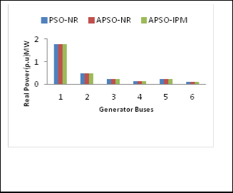
TABLE III
OPTIMAL SETTINGS OF CONTROL VARIABLES WITH LINE LOSS MINIMIZATION
![]()
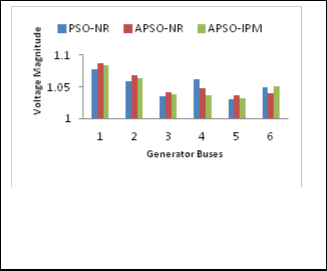
Figure: 1 Real power generation variations with cost minimiza- ![]() tion
tion
![]() Figure: 2 Generator voltage variations with cost minimization.
Figure: 2 Generator voltage variations with cost minimization.
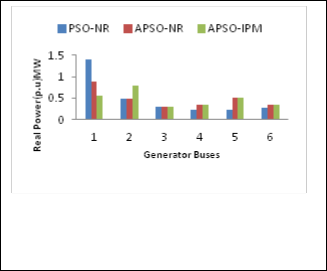
Figure: 3 Real power generation variations with Loss minimiza- tion
IJSER © 2014 http://www.ijser.org
International Journal of Scientific & Engineering Research, Volume 5, Issue 3, March-2014 81
ISSN 2229-5518
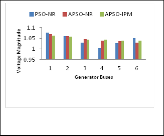
Figure: 4 Generation voltage variations with Loss minimization.
An Adaptive particle swarm optimization algorithm to solve the OPF problem in a power system is presented in this paper. As a representative method of swarm intelligence, APSO sup- plies a novel thought and solution for nonlinear, non- differential and multi-modal problem. For solving the OPF problem, numerical results on the 30-bus system demonstrate the feasibility and effectiveness of the proposed APSO meth- od.
[1] Alsac O, Stott B. “Optimal load flow with steady state security”. IEEE Transactions on Power Apparatus and Systems; vol. PAS-93: pp.745-
51. 1974.
[2] Dommel H, Tinny W. “Optimal power flow solution”. IEEE Transac- tions on Power Apparatus and Systems; vol.PAS-87(10): pp.1866-76.
1968.
[3] Happ HH. “Optimal power dispatch: a comprehensive survey”. IEEE Transactions on Power Apparatus and Systems; vol.PAS-96: pp.841-
54. 1977.
[4] Mamandur KRC. “Optimal control of reactive power flow for im- provements in voltage profiles and for real power loss minimiza- tion”. IEEE Transactions on Power Apparatus and Systems; vol. PAS-
100(7): pp.3185-93. 1981.
[5] Shoults R, Sun D. “Optimal power flow based on P-Q decomposi-
tion”. IEEE Transactions on Power Apparatus and Systems; vol. PAS-
101(2): pp.397-405. 1982.
[6] Habiabollahzadeh H, Luo GX, Semlyen A. “Hydrothermal optimal power flow based on a combined linear and nonlinear programming methodology”. IEEE Transactions on Power Apparatus and Systems; vol. PWRS-492: pp.530-7. 1989.
[7] Burchett RC, Happ HH, Vierath DR. “Quadratically convergent op- timal power flow”. IEEE Transactions on Power Systems; vol. PAS-
103: pp.3267-76. 1984.
[8] Aoki K, Nishikori A, Yokoyama RT. “Constrained load flow using recursive quadratic programming”. IEEE Transactions on Power Sys- tems; vol.2 (1): pp.8-16. 1987.
[9] Abou El-Ela AA, Abido MA. “Optimal operation strategy for reactive power control, Modelling, simulation and control” vol. 41(3).pp.19-
40. AMSE Press, 1992p
[10] Stadlin W, Fletcher D. “Voltage versus reactive current model for dispatch and control”. IEEE Transactions on Power Systems; vol. PAS-101(10): pp.3751-8. 1982.
[11] Mota-Palomino R, Quintana VH. “Sparse reactive power scheduling by a penalty-function linear programming technique”. IEEE Transac- tions on Power Apparatus and Systems; vol.1 (3): pp.31-39. 1986.
[12] Sun DI, Ashely B, Brewer B, Hughes A, Tinney WF. “Optimal power flow by Newton approach”. IEEE Transactions on Power Apparatus and Systems; vol. PAS-103(10): pp.2864-75. 1984.
[13] Santos A, da Costa GR. “Optimal power flow solution by Newton’s method applied to an augmented lagrangian function”. IEEE Proc Generation Transmission Distribution; vol.142 (1): pp.33-36. 1995.
[14] Rahil M, Pirotte P. “Optimal load flow using sequential uncon- strained minimization technique (SUMT) method under power transmission losses minimization”. Electric Power Systems Res; vol.52: pp.61-64. 1999.
[15] Yan X, Quintana VH. “Improving an interior point based OPF by dynamic adjustments of step sizes and tolerances”. IEEE Transac- tions on Power Systems; vol.14 (2): pp.709-17. 1999.
[16] Momoh JA, Zhu JZ. “Improved interior point method for OPF prob- lems”.IEEE Transactions on Power Systems; vol. 14(3): pp.1114-20.
1999.
[17] Lai LL, Ma JT. “Improved genetic algriothms for optimal power flow under both normal and contingent operation states”. Int J Electrical Power Energy Systems; vol.19 (5): pp.287-92. 1997.
[18] Yuryevich J, Wong KP. “Evolutionary programming based optimal power flow algorithm”. IEEE Transactions on Power Systems; vol.14 (4): pp.1245-50. 1999.
[19] Fogel DB. “Evolutionary computation toward a new philosophy of machine intelligence”. New York: IEEE Press, 1995.
[20] J.A. Momoh, L.G. Dias, Guo, and R.A. Adapa, “Economic operation and planning of multi-area interconnected power system,” IEEE Transactions on Power System, vol. 10, pp. 1044-1051, 1995.
[21] S. Granville, J. C. O. Mello, and A. C. G. Melo, “Application of interi- or point methods to power flow, unsolvability,” IEEE Transactions on Power System, vol. 11, pp. 1096–1103, 1996.
[22] Kennedy J. “The particle swarm: social adaptation of knowledge”.
Proc 1997 IEEE International Conference Evolutionary Computation
ICEC, 97, Indianapolis, IN, USA: pp.303-8. 1997.
[23] Angeline P. “Evolutionary optimization versus particle swarm opti- mization”: philosophy and performance differences.Proc 7thAnnual Conference on Evolutionary Programming: pp.601-10. 1998.
[24] Shi Y, Eberhart R. “Parameter selection in particle swarm optimiza- tion”. Proc 7th Annual Conference Evolutionary Programming: pp.591-600. 1998.
[25] Ozean E, Mohan C. “Analysis of a simple particle swarming optimi-
zation system”. Intel Engineering Systems and Artificial Neural
Networks; vol. 8: pp.253-8. 1998.
[26] J. Kennedy, and R. Eberhart, "Particle swarm optimization," IEEE International Conference on NeuralNetworks, vol. 4, pp. 1942-1948, Perth, Australia, 1995.
[27] Y. Shi, and R. C. Eberhart, “A Modified Swarm Optimizer”, In Pro- ceedings of IEEE International Conference on Evolutionary Compu- tation, Piscataway, NJ: IEEE Press, pp.303-308, 1998.
[28] R. C. Eberhart, P. Simpson, and R. Dobbins, Computational Intelli- gence PC Tools: Academic, ch.6, pp. 212–226. 1996.
[29] S. Kirkpatrick, C. D. Gellat, and M. P. Vecchi. “Optimization by Sim- ulated Annealing, Science”. Vol. 220, pp. 671–680, 1983.
[30] M.M. El Metwally, A.A. El Emary, F.M. El Bendary and M.I. Mosaad. “Optimal Power Flow Using Evolutionary Programming Tech- niques.” MEPCON’2008 Power Systems, pp. 260-264, 2008.
IJSER © 2014 http://www.ijser.org
International Journal of Scientific & Engineering Research, Volume 5, Issue 3, March-2014 82
ISSN 2229-5518
BIOGRAPHIES

Leela Prasad.T is purusing his M.Tech (Power System Automation and Control) in the Department of Electri- cal & Electronics Engineering, from P.V.P.Siddhartha Institute of Technology, Vijayawada, Andhra Pradesh, India. He obtained B.Tech degree in Electrical and Electronics Engineering from J.N.T.U Kakinada in the year 2009.

Vijaya Anand Nidumolu received his B. E in Electrical Electronics engineering obtained his M.E in Power Sys- tems & Automation from Andhra university in year 2002. His area of interest are model order reduction, interval systems analysis and power system operation & control. Presently he is Associate Professor, EEE pvpsit, vijay- awda.

Dr.Ch.Padmanabha Raju is currently working as Professor in the Department of Electrical & Electron- ics Engineering, P.V.P.Siddhartha Institute of Tech- nology, Vijayawada, and Andhra Pradesh, India. He obtained Ph.D from J.N.T.University, Kakinada .His areas of interest are Power System Security, OPF techniques, Deregulation and FACTS.
.
IJSER © 2014 http://www.ijser.org