Where is the rating of the alternative with respect
to the criterion
International Journal of Scientific & Engineering Research, Volume 4, Issue 12, December-2013 2157
ISSN 2229-5518
Handoff between heterogeneous networks based on MADM methods
G.A.Preethi, Dr. C. Chandrasekar, N.Priya
Delay and Cost of the network has been used for analyzation.
.
—————————— ——————————
Wireless mobile is not only used for communica- tion, also used for data transfer, video conferenc-
This paper consists of Section II Related work, III dis- cusses about MADM Methods IV is the Efficiency ana-
IJSER
ing, net-surfing etc,. For all these utility, high
bandwidth and rapid transfer of data is needed. In case
of mobility of a wireless device, signal reception will be
a challenge in dense areas. In this juncture it is recom-
mended to afford different networks. Each network will
have a range of coverage. When a wireless node moves beyond its cell-limitation, it should change over to
another base station which belongs to different network. Since its old network no longer supports it. This is termed as heterogeneous-handoff. In the event of Hori- zontal handoff, which involves the same network, Re- ceived signal strength measure is the only significant thing to consider. For the heterogeneity , we need to analyse different parameters such as bandwidth, delay, Signal to Noise ratio etc,. We should also consider the User preferences such as wide coverage, low cost, secu- rity etc,. When a user using a low-cost network is handed over to another high-cost network, then it will be an issue. So we have to analyse different types of is- sues while considering heterogeneous network. In [4] we have compared two MADM methods such as TOP- SIS and AHP for handoff decision. In this paper we have related ELECTRE and GRA methods with TOPSIS and also extended our work for efficiency analyzation and measurements of bandwidth, end-to-end delay for the networks.
————————————————
G.A.Preethi is currently pursuing phd in Computer Science in Periyar
University, Salem,Tamilnadu,INDIA. E-mail: preethi_ga2005@yahoo.com
Dr. C.Chandrasekar is an Associate Professor in Periyar University, Sa- lem, TamilNadu, INDIA. E-mail: ccsekar@gmail.com
lyzation, V Simulation output and Discusssion. Finally
Section VI concludes the work.
Faouzi zarai et al [3] formulated a new architecture for handoff decision making which considers the resource utilization and the user preference for the network. Hui zeng et al [5] approach was based on integrated frame- work through multi-layer. The proposed algorithm pro- vides a holistic handoff solution to the ad-hoc networks. Hyun-ho choi et al [6] presented scheme which requires a pre-registration and pre-authentication of networks before handoff. It also used packet buffering procedure for preventing the packet loss. Lahby Mohammed et al [7] gave a different approach by combining the ANP and TOPSIS methods. Their approach also given by con- sidering and eliminating the differentiated weights of criterions and history attributes for handoff. Nirmala Shenoy [8] presented a framework for seamless roaming which overlays network comprising of Inter-System Interface Control Units (IICU) to support inter-network communication and control for Location Management. It optimizes the call delays, traffic and other QOS para- meters. Y.Wu et al [10] experimented a congestion aware vertical handoff which reduced the packet loss and delay.
The MADM method is based on ―GRA‖,
―ELECTRE‖ and ―TOPSIS‖ however we apply it in a
distributed manner. Thus, we place the computing
IJSER © 2013
International Journal of Scientific & Engineering Research, Volume 4, Issue 12, December-2013 2158
ISSN 2229-5518
processing in the visited networks rather than on the mobile terminal. MADM allows the mobile terminal to choose the ―best‖ network towards which it will be con- nected.
Construction of the decision matrix: the decision matrix is expressed as
Here,
d11 ..
d1m
Candidate networks are A1, A2, and A3
Criteria are X1, X2, and X3
Calculates Voice Application
D ..
d n1
.. ..
.. d nm
In this section illustrating the usage of the selected me- thods and the results are compared,
TABLE 1: MEASURES OF ALTERNATIVES BASED ON CRITERIA.
![]()
![]()
Where is the rating of the alternative with respect
to the criterion ![]()
![]()
Construct the normalized decision matrix: each element is obtained by the Euclidean normalization
rij
![]()
d ij
2
i 1 ij
(1)
0.512
rij 0.767
0.602
0.622
0.421
0.842
IJSER
0.384
0.502
0.337
User preference for Voice application is also converted to crisp numbers and normalized so that is equal to 1. The normalized preference, i.e. the weighting factors for the voice Wv application is:
Construct the weighted normalized decision matrix
Assume a set of weights for each criteria w j for j=1....n
Wv 0.4
0.3
0.3
Multiply each column of the normalized deci- sion matrix by its associate weight
In this proposed method the TOPSIS (Technique for Or- der Preference by Similarity to Ideal Solution) is taken
The weighted normalized decision matrix vij is computed as
and it is analysed. This method considers three types of attributes,
Qualitative benefit attributes/ criteria
vij
w j * rij
0.205
0.181
0.126
Quantitative benefit attributes
Cost attributes
vij 0.307
0.154
0.187
0.151
0.253
0.101
The basic principle of the TOPSIS is that the chosen al- ternative should have the shortest distance from the positive ideal solution and the farthest distance from the negative ideal solution. TOPSIS[4] method is used to
Determine the positive ideal solution and negative ideal solution
Positive ideal solution
select the network that satisfies the given criteria after
A* {v* ...v* } {(max v
| j J ),
performing six sequential steps listed below. The net-
work with maximum value from the rank order is the
one that is close to the positive ideal solution and far
(min i
1
vij
n
| j J ' )}
i ij
away from the negative solution. The criteria for select- ing the network are maximum bandwidth, handoff sig- naling delay, battery and minimum cost.
i 1..3,
j 1..3
(2)
IJSER © 2013
International Journal of Scientific & Engineering Research, Volume 4, Issue 12, December-2013 2159
ISSN 2229-5518
Negative deal solution
A' {v ' ...v ' } {(min v
| j J ),
d11 ..
d1m
(max i
1
vij
n
| j J ' )}
i ij
D
..
d n1
.. ..
.. d nm
i 1..3,
j 1..3
(3)
A* 0.307
A' 0.154
0.187
0.151
0.253
0.101
Step 2: Construct the normalized decision matrix: each element ![]() is obtained by the min, max Method norma- lization
is obtained by the min, max Method norma- lization![]()
For bandwidth attribute, the normalized value of is computed as:
Calculate the similarity distance measures for each al-
d ij
ternative.
Similarity distance from the positive ideal al-
ternative is :![]()
rij max (6)
d j
For delay and cost attribute, the normalized![]()
*
i i 1
* 2
1 ij
j 1..m
(4)
value of rij is computed as:
min
![]()
Similarity distance from the negative ideal al- ternative is :
m
rij
d j
![]()
d ij
(7)
S '
i 1
(vij
v ' ) 2
j 1..m
(5)
0.666
0.833
0.800
S * 0.163 0
0.219
rij 1
0.806
0.400
IJSER
S ' 0.064
0.219
0.011
0.500 1 1
i
Ranking : Calculate the relative closeness to the
S '
matrix
Assume a set of weights for each criteria w j
for j=1....n![]()
ideal solution C *
j
S * S '
. For the voice
Multiply each column of the normalized deci-
sion matrix by its associate weight
application,
C * 0.281
j
0.589
j
0.047
v
The weighted normalized decision matrix ij is
computed as
To rank a set of alternatives, the ELECTRE method as
vij
w j * rij
0.266
0.249
0.240
outranking relation theory was used to analyze the data of a decision matrix. The Elimination and Choice Trans- lating Reality (ELECTRE) method was the most exten- sively used outranking methods reflecting the decision
vij 0.400
0.200
0.242
0.300
0.120
0.300
maker’s preferences in many fields. The ELECTRE I ap- proach was then developed by a number of variants. We have ELECTRE II, III, V and many types. ELECTRE me- thod reflects the dominance of relations among alterna- tives by outranking relations[2].
Step 4: To find the concordance and discordance inter- val sets , Let M= {a,b,c,….} denote a finite set of alterna- tives, in the following formulation we divide the attribute sets into two different sets of concordance in- terval set C pq and discordance interval set D pq .
C pq
{ j | x pj
xqj }
sion matrix is expressed as
Dpq { j | x pj xqj }
IJSER © 2013
International Journal of Scientific & Engineering Research, Volume 4, Issue 12, December-2013 2160
ISSN 2229-5518
1 1
C pq
jC W j
F 0
0
The concordance matrix can be framed as
...
c(1, m)
1 0
C
...
...
...
c(m,1)
...
...
Let Ca
and Da
be the net superior and net inferior
0
0.4
value respectively.
Ca sums together the number of
C 0.7 0
competitive superiority for all alternatives, and the more
and bigger, the better. The Ca is given by:
0.3
0.6 n n
Ca b1 C( p, q) b1 C(q, p)
C1 0.4 1 0.6
(12)
m m
![]()
C p1 q1 C( pq) / m(m 1)
![]()
C 0.333
(8)
C2 0.7 0.6 0.1
C3 0.9 0.4 0.5
Here ![]() is the critical value, which can be determined by average dominance index. Thus, a Boolean matrix (E) is
is the critical value, which can be determined by average dominance index. Thus, a Boolean matrix (E) is
given by:
On the contrary, d a is used to determine the number of inferiority ranking the alternatives:
n n
![]()
e( p, q) 1, C( p, q) x C
d a b1 d ( p, q) b1 d (q, p)
(13)
IJS(9) ER
![]()
e( p, q) 0, C( p, q) C
d1 0.027
E 1
1
0 1
0
1
d 2 0.104
d 3 0.077
Smaller is better. This is the biggest reason that smaller net inferior value gets better dominant than larger net
max[ v pj vqj ] jD
![]()
d ( p, q) pq
max[| v pj vqj |] jD
(10)
inferior value by sequence order.
The main procedure of GRA[9] is firstly translating the performance of all alternatives into a comparability se-
d (1, m)
quence. This step is called grey relational generating.
According to these sequences, a reference sequence
D
d (m,1)
(ideal target sequence) is defined. Then, the grey rela- tional coefficient between all comparability sequences and the reference sequence is calculated. Finally, base on
0.896
0.85
these grey relational coefficients, the grey relational grade between the reference sequence and every compa-
D 1
1
rability sequences is calculated. If a comparability se-
0.775 1
quence translated from an alternative has the highest
grey relational grade between the reference sequence
and itself, that alternative will be the best choice. The procedures of grey relational analysis are shown in Fig![]()
m m
d p1 q1 C( pq) / m(m 1)
![]()
d 0.919
(11) 1.
Here ![]() is the critical value, which can be determined byaverage dominance index. Thus, a Boolean matrix (F) is given by:
is the critical value, which can be determined byaverage dominance index. Thus, a Boolean matrix (F) is given by:
IJSER © 2013
International Journal of Scientific & Engineering Research, Volume 4, Issue 12, December-2013 2161
ISSN 2229-5518
Grey Relation Generating![]()
x 1
yij
y*
(Comparability Sequence)
ij Max{Max{y
, i 1...m} y* , y* Min{y
, i 1...m}}
ij ij ij ij
for i = 1…m, j = 1…n (16)
Create a Reference Sequence.
Grey Relation Co-efficient Cal- culation.
Eq. (14) is used for the-larger-the-better attributes, Eq. (15) is used for the-smaller-the-better attributes and Eq.(16) is used for the closer to the desired value.
After the grey relational generating procedure using Eq. (14), (15) or Eq. (16), all performance values will be scaled into [0, 1]. For an attribute j of alternative i, if the
value
xij which has been processed by grey relational
Grey Relation Grade Calcula- tion.
generating procedure, is equal to 1, or nearer to 1 than the value for any other alternative, that means the per- formance of alternative i is the best one for the attribute j. Therefore an alternative will be the best choice if all of its performance values are closest to or equal to 1. How- ever, this kind of alternative does not usually exist. This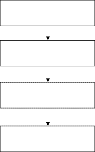
Fig 1 : Procedure of Grey Relational Analysis.
paper then defines the reference sequence
X 0 as
(x01, x02 ,...x0 j ,...xon ) (1,1,...1,...1) and then aims to
When the units in which performance is measured are different for different attributes, the influence of some attributes may be neglected. This may also happen if some performance attributes have a very large range. In
find the alternative whose comparability sequence is the
closest to the reference sequence.
Grey relational coefficient is used for determining how
addition, if the goals and directions of these attributes
close
xij
is to
x0 j . The larger the grey relational coeffi-
are different, it will cause incorrect results in the analy-
sis [9]. Therefore, processing all performance values for
cient, the closer
xij and
xoj . The grey relational coeffi-
every alternative into a comparability sequence, in a
cient can be calculated by Eq. (4).
process analogous to normalization, is necessary. This
x x
min max
processing is called grey relational generating in GRA. For a MADM problem, if there are m alternatives and
( 0 j ,
ij )
ij
![]()
max
n attributes, the i th alternative can be expressed as
for i 1,...m, j 1,...n
(17)
Yi ( yi1 , yi 2 ,...yij ,..yin ) where
yij
is the perfor-
In Eq. (17), ( x0 j , xij ) is the grey relational co-efficient
mance value of attribute j of alternative i . The term
between
x0 j and
xij. and
Yi can be translated into the comparability sequence
ij
![]()
![]()
xoj xij ,
X i (xi1 , xi 2 ,...xij ,..xin ) by use of one of equations
1,2,3.
min
max
Min{i 1,...m; j 1,...n},
Max{i 1,...m; j 1,...n},
xij
![]()
yij Min{yij , i 1...m}
Max{yij , i 1...m} Min{yij , i 1...m}
is the distinguishing co-efficient, [0,1] .
The purpose of the distinguishing coefficient is to ex-
for i = 1…m, j = 1…n (14)
Max{yij , i 1...m} yij
pand or compress the range of the grey relational coeffi- cient. After grey relational generating using Eq. (14),(15)![]()
xij
Max{yij , i 1...m} Min{yij , i 1...m}
or (16),
max will be equal to 1 and
min will be equal
for i = 1…m, j = 1…n (15)
to 0. Fig. 2 shows the grey relational coefficient results
when different distinguishing coefficients are adopted.
IJSER © 2013
International Journal of Scientific & Engineering Research, Volume 4, Issue 12, December-2013 2162
ISSN 2229-5518
In Fig. 2, the differences between ( x0 j , x pj ),
TABLE: 3 GREY RELATIONAL CO-EFFICIENT
( x0 j , xqj )
and
( x0 j , xrj ) always change when dif-
ferent distinguishing coefficients are adopted. In our paper, we have kept the distinguishing co-efficient as
0.5.
The Grey Relational Grade can be calculated by Eq.(18)
n
( X 0 , X i ) w j ( x0 j , xij )
j 1
for i = 1,…m (18)
From the above Table:3 we have measured the co- efficient values based on 0.5. From the Fig:2 we assign
0.1 as distinguishing co-efficient value, then wifi band-
In Eq.(18),
( X 0 , X i ) is the grey relational grade be-
width as well as delay has decreased heavily. And cost
tween
X 0 and
X i . The level of correlation between
has increased, so it will not be a good option to choose.
reference sequence and comparability sequence has
Wimax has the highest value for bandwidth and its
transmission delay and cost has little decrease. UMTS
been represented. The weights has been given by
w j .
has decreased bandwidth , increased delay and cost. So
The grey relational grade represents the degree of simi- larity between the comparability sequence and the refer- ence sequence. The Reference sequence represents the
best attribute by among the comparability sequence. If a
here comes Wimax as the best option for handoff selec- tion when compared to other networks.
comparability sequence gets the highest grey relational grade with the reference sequence, then that will be the best choice.
Calculating the Grey Relational Reference for the net- works
For Wifi
xij
20 15 ,
30 15
xij 0.333 , Likewise we
calculate for each and every alternative.
TABLE:2 GREY RELATIONAL REFERENCE SEQUENCE
Bandwidth (X1) | Delay (X2) | Cost (X3) | |
Wifi (A1) | 0.333 | 0.166 | 0.833 |
Wimax (A2) | 1 | 0 | 0 |
UMTS (A3) | 0 | 1 | 1 |
We have assumed our distinguishing co-efficient as 0.5. Anyhow we have calculated for different values and analyzed the results.
Fig 2: Grey relational co-efficient ( distinguishing co-efficient 0.1 )
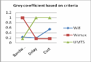
Fig 3: Grey Relational co-efficient (Distinguishing co-efficient 0.2)
IJSER © 2013
International Journal of Scientific & Engineering Research, Volume 4, Issue 12, December-2013 2163
ISSN 2229-5518
From the Fig: 3 Wimax has higher bandwidth , lesser delay and cost. UMTS bandwidth is very low and its delay and cost has increased very highly. Wifi cost shows increased rank, bandwidth and delay are compa- ratively very low rank. From Fig:4 and Fig:5, the Grey relational grade for Wimax has shown augment result with higher value and considerably diminished values of delay and cost. Both wifi and UMTS has lesser meas- ures for Bandwidth and higher measures for delay and cost.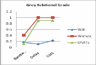
quence is closer to the comparability sequence in band- width criteria. Thus it is the best option for handoff , but its delay and cost shows higher values in which it should be lesser the better. Wifi delay and cost is lesser compared to other two alternatives. But it does not have larger coverage, thus it needs too many handoffs which is not a good option. UMTS results are not considerable here since it shows poor measures still its delay and cost is average.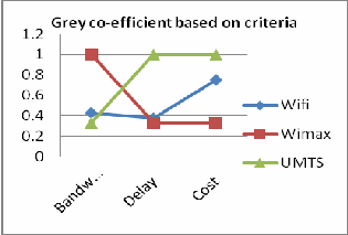
Fig: 6 Grade based on criterion weights.
IJSER
Fig 4: Grey Relational co-efficient (Distinguishing co-efficient 0.5)
Fig 5: Grey Relational co-efficient (Distinguishing co-efficient 0.7)
Fig 5: Grey Relational co-efficient (Distinguishing co-efficient 0.7)
TABLE:4 GREY RELATIONAL GRADE.
Bandwidth | Delay | Cost | |
Wifi | 0.1712 | 0.1122 | 0.2247 |
Wimax | 0.4 | 0.999 | 0.999 |
UMTS | 0.1332 | 0.3 | 0.3 |
From the above Table:4, we have obtained the grey rela- tional grade for all the alternatives by propagating with their corresponding weights. Wimax reference se-
From the above Fig:6, the grey relational grade values
are represented by multiplying the criterion co-efficient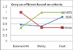
values with their corresponding weights. Eventhough the delay and cost of the Wimax is increased, it shows good performance for bandwidth while compared with other alternatives.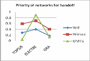
Fig: 7 Comparison of MADM measures.
From the above Fig:7, the ELECTRE method shows high values for UMTS network. These measures are based on Concordance value. For TOPSIS and GRA, Wimax shows higher values for handoff decision making. So, Wimax can be selected as a better choice for roaming after successful handoff. In another aspect, TOPSIS and ELECTRE shows higher values for Wifi and Wimax
IJSER © 2013
International Journal of Scientific & Engineering Research, Volume 4, Issue 12, December-2013 2164
ISSN 2229-5518
compared to GRA. Though GRA method is efficient while compared with TOPSIS and ELECTRE. Whilst in terms of MADM methods, ELECTRE and TOPSIS me- thods are time consuming. GRA method is efficient compared with other 2 methods.
All the three methods efficiency has been analyzed. For analyzing a method’s efficiency, we need to know what are all its basic operations [1], how much time it takes to
execute and how many times it repeats the basic opera-
tion to get the required output. Based on the input size
Finally we get,
T (n) cm
M (n) ca
A(n) cd
D(n)
the efficiency will get affected. First we take TOPSIS
method. Find its basic operations. In the first step, input
where
cm represents one multiplication,
ca represents
is 3X3 matrix 9 numbers. Output: 3 numbers.
one addition and
cd represents one division.
d ij
, Normalize the given matrix.
M (n), A(n)andD(n) represents Multiplication , Ad-
![]()
ij m
dition and Divisions respectively.
T (n) represents ap-
d ij
i 1
Here Division and Square root operation performed 9 times.
proximate time efficiency of the algorithm.
vij
w j * rij , Weighted normalized decision
tions , 9 Divisions and 3 Comparisons.
IJSER
matrix is calculated. Multiplication 9 times.
Step3: A* {Max v
| Mini vij } ,
accomplish 18 additions, 18 Multiplications and 9
A' {Min v
| Maxi vij
}. Calculate Maximum and
Divisions.
Minimum values for each column. Here we compare 6 times.
m m
* * 2 ' ' 2 ,
![]()
![]()
i 1
i 1
ULATION OUTPUT AND DISCUSSION
Measure Positive and Negative ideal solutions. Square root and Subtraction performed 18 times.
S '
![]()
j
S * S '
, Calculate the relative closeness
j j
to the ideal Solution. Division and Addition operations performed 3 times.
d ij
![]()
Step 2: Normalized Decision Matrix rij Ma x
d j
for
Bandwidth,
rij
Min
![]()
j
d ij
for Delay and Cost. Here we do
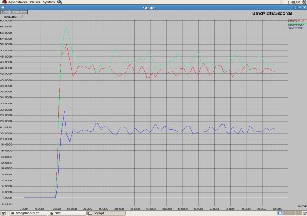
Fig: 8 Bandwidths of Networks
9 comparisons, 9 division operations.
IJSER © 2013
International Journal of Scientific & Engineering Research, Volume 4, Issue 12, December-2013 2165
ISSN 2229-5518
From the above Fig:8, Wimax throughput is slightly higher compared with WLAN. UMTS shows low bit- rate. The Throughput mainly depends on the data rate, since wimax supports higher data rate it gets acceptable results. All the three networks simulation executed at same time and the data transfer rate is set as 2MB. Simu- lation topology is set on 500X500 geometry. The Mobile node sends request to all three networks such as WLAN, Wimax and UMTS when its signal range goes down the threshold value. It Handovers to the network which fullfills its requirements.
network side, Wimax and on the Decision making scheme GRA gives optimum results. In our future work we will consider packet delivery ratio and analyze about the packet drops.
[1] Anany Levitin, ― Introduction to the Design and Analysis of Al-
gorithms ―, 3rd Edition. Pearson Publications , p.p 41-50, 2012.
[2] Ermatita et al,. ―MADM Methods in Solving Group Decision Support System on Gene Mutations Detection Simulation‖ In- ternational Conference on Distributed Framework and Applica- tions (DFmA), 2-3 Aug. 2010. pp.1-6. Yogyakarta
[3] Faouzi zarai et al,. ―Seamless Mobility in Heterogeneous Wire- less Networks‖, International Journal of Next Generation Net- work(IJNGN), Volume 2, No 4, Dec 2010.
[4] G.A. Preethi, Dr. C. Chandrasekar, ―Seamless Mobility of Hete- rogeneous Networks on TOPSIS and AHP methods‖, National Conference on Computer and Communication Technology, Eswari Engineering College, Chennai, 5th and 6th May 2011.
[5] Hui zeng et al,. ―A Multi Layer approach for Seamless Soft Handoff for Mobile Ad Hoc Networks‖ , IEEE Globecom Workshops 2010, Dec 6-10, Miami , Florida, USA.
[6] Hyun-ho choi et al,. ― Seamless Handoff Scheme based on Pre- registration and Pre-authentication of UMTS-WLAN inter- working‖ , Wireless Personal Communications, Springer 2007.
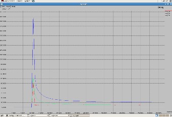
Fig: 9 End-to-end Delay of Networks.
From the above Fig:9, UMTS shows very high delay re- lated to other two networks. Here WLAN shows low delay since its coverage area is small and bandwidth is comparitvely high. Based on the simulation results and MADM methods measurements, Wimax Shows opti- mum output for Handoff Decision. In the aspect of effi- ciency, that is the number of operations performed and the number of times measured, ELECTRE Method has minimum estimations to be performed while GRA and TOPSIS has numerous calculations. If we take many networks and parameters, the rate of basic operation will reduce gradually.
Habitually mobile nodes will undergo horizontal han- doff. In case of coverage problems it will have informa- tion about its nearby service providers. In our case we have taken 3 different networks and analyzed its per- formance based on simulation results. And for handoff decision making we have taken 3 different MADM me- thods to investigate and wrap up the network which gives favourable outcomes for handoff. We have ana- lyzed about the efficiency of MADM methods in which ELECTRE method is efficient, But on the other hand it shows totally different measures for networks. In the
Volume 41. pp. 345-364.
[7] Lahby Mohammed et al,. ―An Intelligent Network Selection Strategy Based on MADM Methods in Heterogeneous Net- works‖ , International Journal of Wireless and Mobile Net- works(IJWMN), Volume 4, No 1, Feb 2012.
[8] Nirmala shenoy, ― A Framework for Seamless Roaming Across Heterogeneous Next Generation Wireless Networks‖ , Wireless Networks, Volume 11, pp. 757-774, Springer science 2005.
[9] Yiyo Kuo et al, ―The use of grey relational analysis in solving multiple attribute decision-making problems‖ Elsevier Publica- tions, Volume 55, Issue 1, August 2008, pp. 80–93.
[10] Y.Wu et.al,. ―Congestion-aware proactive vertical handoff algo- rithm in heterogeneous wireless networks‖, IET communica- tions, Vol. 3, Issue 7, 2009, pp. 1103–1114
IJSER © 2013