International Journal of Scientific & Engineering Research, Volume 4, Issue 8, August-2013 1711

ISSN 2229-5518

Formulation for Second Derivative of Generalized

Delta learning Rule in Feed Forward Neural Networks for Good

Generalization

1 Shivpuje Nitin Parappa 2 DR. Manu Pratap Singh

Dept. of Comp. Sci. Institute of Computer & Information Science
Balaghat Polytechnic, Ahmedpur Dr. B.R.Ambedkar University, Agra-282002
Dist: Latur (MS) 413515 Uttar Pradesh, India
(e-mail: shivpujenitin@gmail.com) (e-mail: manu_p_singh@hotmail.com)

Abstract— Generalized delta learning rule is very often used in multilayer feed forward neural networks for accomplish the task of pattern mapping. A backpropagation learning network is expected to generalize from the training set data, so that the network can be used to determine the output for a new test input. This network uses the gradient decent technique to train the network for generalization. It evolves the iterative procedure for minimization of an error function, with adjustments to the weights being made in a sequence of steps. The first derivate of the error with respect to the weights identifies the local error surface in decent directions. Therefore for every different presented pattern, the network exhibits the different local error and the weights modify in order to minimize the current local error. In this paper, we

are providing the generalized mathematical formulation for the second derivative of the error function for the arbitrary feed forward neural network topology. The new global error point can evaluate with the help of current global error and the current minimized local error. The weight modification process accomplishes two times, one for the present local error and second time for the current global error. The proposed method indicates that the weights, these are determines from the minimization of global error are more optimal with respect to the conventional gradient decent approaches.

Index Terms — Generalization, Pattern mapping networks, Back propagation learning network, decent gradient, and Conjugate descent.

1 INTRODUCTION

——————————  ——————————
Generalization is different from interpolation, since in generaliza- tion the network is expected to model the unknown system or function from which the training set data has been obtained. The problem of determination of weights from the training set data is known as the loading problem [1]. The generalization perfor- mance depends on the size and complexity of the training set, be- sides the architecture of the network and the complexity of the problem [2]. Therefore, if the performance for the test data is as good as for the training data, then the network is said to have generalized from the training data. The feed forward neural net- work architecture is more commonly used to perform the task of generalization with pattern mapping network. In this pattern mapping network for generalization the algorithm for modifying the weights between the different interconnected layers is usually known as back propagation learning technique [3]. This algorithm is a supervised learning method for multi layered feed forward neural networks. It is essentially a gradient descent local optimiza- tion technique which involves backward error correction of net- work weights. It evaluates the derivatives of the error function with respect to weight in weight space for any given presented input pattern from the given training set [4]. It involves the itera- tive procedure for minimization of an error function, with adjust- ment to the weights being made in a sequence of steps. In each steps we can distinguish between two distinct stages. In the first stage, the derivatives of the error function with respect to the weights must be evaluated. In the second stage, the derivatives are then used to compute the adjustment to be made to the weights [10]. The first stage process, namely the propagation of errors backward through the network in order to evaluate deriva-
tives, can be applied to many other kinds of network and not just the multi layer perceptron. It can also be applied to the error func- tions other than just the simple sum-of-squares, and the evalua- tion of other derivatives such as the Jacobin and Hessian metrics [11] and also, the second stage of weight adjustment with the cal- culated derivatives can be tackled using a verity of optimization schemes.
Despite the general success of back-propagation method in the learning process, several major deficiencies are still needed to be solved like convergence guarantee and convergence rate, nature of error, ill posing and over training. The convergence rate of back-propagation is very low and hence it becomes unsuitable for large problems. Furthermore, the convergence behavior of the back-propagation algorithm depends on the choice of initial val- ues of connection weights and other parameters used in the algo- rithm such as the learning rate and momentum term. There are various other enhancements and modifications were also present- ed by different researchers [5-7] for improving the training effi- ciency of neural network based algorithms by incorporating the selection of dynamic learning rate and momentum [8-9]. The im- provement in performance of back propagation is further consider with the evaluation of the Jacobin matrix [12], whose elements are given by the derivatives of the network outputs with respect to the inputs. The Jacobin matrix provides a measure of the local sensitivity of the outputs to change in each of the input variables. In general, the network mapping represented by a trained neural network will be non-linear, and so the elements of the Jacobin ma- trix will not be constant but depends on the particular input vec- tor used.

IJSER © 2013 http://www.ijser.org

International Journal of Scientific & Engineering Research, Volume 4, Issue 8, August-2013 1712

ISSN 2229-5518

The back propagated error is further used to evaluate the second derivatives of the instantaneous squared error. These derivatives form the elements of the Hessian matrix [13], which involves the basis of a fast procedure for re-training a feed forward network following a small change in the training data. Thus, due to the several applications of the Hessian matrix, there is various ap- proximation schemes have been used to evaluate it like the diago- nal approximation [14] outer product approximation and inverse Hessian [15]. The exact evaluation of the Hessian matrix has also proposed, which is valid for a network of arbitrary feed forward topology. This method is based on an extension of the technique of the back propagation used to evaluate the first derivatives, and shares the many desirable features of it [16]. The second derivative of the error with respect to weight is obtained as conjugate de- scent method [17, 18]. The further improvement in conjugate de- scent method is also considered [19] and in the family of Quasi – Newton algorithms [20]. Further, the influence of gain was studies by few researchers [21 – 23]. The gain parameter controls the steepness of the activation function. It has been shown that a larg- er gain value has an equivalent effect of increasing the learning rate. Recently it has been suggested that a simple modification to the initial search direction, i.e. the gradient of error with respect to weights, can substantially improve the training efficiency. It was discovered that if the gradient based search direction is locally modified by a gain value used in the activation function of the corresponding node, significantly improvements in the conver- gence rates can be achieved [24].
In this present paper, we are considering a multilayer fed forward neural network with a training set of English alphabets. This neu- ral network is trained for good generalization with generalized second derivative delta learning rule for the stochastic error. This random error is back propagated among the units of hidden lay-

involves determining these weights, for the given training input- output pattern pairs as shown in figure 1.

Figure 1: Architecture of the multi layer feed forward Neural

Network

So far, in order to determine the weights in supervisory mode it is necessary to know the error between the derived or expected out- put and the actual output of the network for a given training pat- tern. We know the desired output only for the units in the final output layer, not for the units in the hidden layers. Thus, the same error of output layer is back propagated for the hidden layers to guide the updating or modification in the weights. Therefore, the instantaneous error can minimize by updating the weights be- tween the input layer to hidden layer and hidden to output layer. Thus, we use the approach of gradient descent along the error surface in the weights space to adjust the weights to arrive at the optimum weight vector. The error is defined as the squared dif- ference between the desired output and the actual output ob- tained at the output layer of the network due to application of an input pattern from the given input-output pattern pairs. The out- put has calculated using the current setting of the weights in all the layers as follows:

n

ers, for the modification of the connection weights in order to min- imize the error. This modification in the weights is preformed with generalized second derivative of error with respect to weights between hidden layer and output layer and also in be-

y k = f (∑ Z iWi k )

i =1

Where f the output function, Zi

(2.1)

is the output of hid-

tween input and hidden layer. The neural network is trained for capturing the generalized implicit functional relationship between input and output pattern pairs. Thus, it is expected from the adap-

den layer and

output layer.

Wi k

is the weight between hidden and

tive neural network is that it could able to recognize the individu-
al characters from the handwritten English word of three letters.

And , also for hidden layer’s processing unit output ;

n

Hence, the proposed method is providing the generalized way for minimization of optimal global error which consists with instan-

Z i =

f (∑Vi j X j )

j =1

(2.2)
taneous unknown minimum local errors.

Where

X j the output of input is layer and

Vi j

is the

2. FEED FORWARD NEURAL NETWORK WITH DELTA LEARN- ING RULE

weight between input and hidden layer.

The instantaneous squared error for the lth pattern can represent as:

A multi layer feed forward neural networks normally consist with the input, output and hidden layers. The processing units in the

E l = 0.5∑[t

k

− yk ]

(2.3)
output layer and hidden layers usually contain non linear differ-

Where tk

is desired output.

entiable output function and the units of input layer use the linear
output function. If the units in the hidden layers and in the output
layer are non-linear, then the number of unknown weights or
connection strengths depend on the number of units in the hidden
layers, besides the number of units in the input and the output
layers. Obviously, the network is suppose to use for generaliza- tion i.e. pattern mapping. Thus, the pattern mapping, problem
Thus, for each input-output pattern pair the network has the dif- ferent error. So, we have the local errors for the given input- output pattern pairs.
The weights are updated to minimize the current local error or
unknown instantaneous square error for each presented input-
output pattern pair. Thus, the optimum weights may be obtained

IJSER © 2013 http://www.ijser.org

International Journal of Scientific & Engineering Research, Volume 4, Issue 8, August-2013 1713

ISSN 2229-5518

if the weights are adjusted in such a way that the gradient descent is made along the total error surface. The error minimization can be shown as;
put pattern. It is easy to interpret that, every time the network tries to minimize the current local unknown error. Now, it is clear that in descent gradient learning rule weights of the network are

∂E l

∂Wi k

= [t k − yk ] f

( yk ) zi

(2.4)
updating only on the basis of local error rather than the global
error and in order to obtain the generalized behavior the updating
in the weights are required along the descent gradient of the glob-

Weights modifications on the hidden layer can be de-

fined as;

al error or least mean square error for the entire training set.
Hence, it can realize that to obtain the good generalization for the

∆Vij

= ∂E l

∂V

= ∑ ∂k * (∂yk

)[t k

− yk ] f

( yk

) zi

(2.5)
given input output pattern pairs the weight updating should take
place for the global error rather than the local error surfaces.

ij k ij

'

Therefore, we can visualize a k- dimensional error surface in
[Let, ∂k = [t k
And we have

− y k ] f

'

( yk ) ]

which we have different descent gradient corresponding to differ-
ent input output pattern pairs, but only one descent gradient will
activate at a one time. So, it is difficult to keep the entire local de-

∆Vij = ∑ ∂k *Wi k f

k

( zi )

(2.6)
scent gradients and to search for the global one. Instead of this, we
can keep the different minima points of the error corresponding to

Thus the weight updates for output unit can be repre-

sented as;

different input output pattern pairs. These minima points will distribute in the entire error surface and to trace the global mini-

Wik (t + 1) = Wik (t ) + η ∆Wi k (t ) + α ∆Wi k (t − 1)

Where

Wik (t ) is the state of weight matrix at iteration t

(2.7)
ma from these local minimum points will easy and convenient. Thus, to accomplish the determination of local minimum points, we can consider the second derivative of descent gradient of the local errors.

Wik (t + 1) is the state of weight matrix at next iteration

3. GENERALIZED SECOND DERIVATIVE FOR FEED FORWARD

Wik (t − 1)

tion.

∆Wi k (t )

is the state of weight matrix at previous itera-

is current change/ modification in weight ma-

MULTILAYER NEURAL NETWORKS:

In this section we present a generalized method for obtaining the second derivative of the descent gradient of global error with re- spect to weight in weight space for the good generalized behavior

trix and α is standard momentum variable to accelerate

learning process.

This variable depends on the learning rate of the net- work. As the network yields the set learning rate the momentum variable tends to accelerate the process.

In this process the weights are updating on each step for the in- stantaneous local unknown square error instead of least mean error or total error or global error for the entire training set. The determination of the total error surface cannot be known, because the set of input-output pattern pairs is large and continuous. Thus, the gradient descent on each step is obtained along the in- stantaneous local error surface. Hence the weights are now ad- justed in a manner that the network is leading towards the mini- ma of local error surface for the presented input-output pattern
of the feed forward multilayer neural network for the given train- ing set. Therefore to obtain the optimal weight vector for the feed forward neural network, the weight modification should perform for the global minimum point among the various local error min- ima points. Thus, the modification in the weight vector in each step is for minimizing first the local instantaneous square error and in second step is to minimize the current global or least mean square error. Now, we illustrate the generalized method for de- termining the second derivative of instantaneous error and further for the current global error correspond to presented input-output pattern pairs on each step. The error can obtain for the feed for- ward neural network as shown in fig (1) for the lth pattern from the equation (2.3) and decent gradient for the instantaneous square error as obtained from the equation (2.4). Now from these
two equations we have;
pair. Therefore to obtain the optimum weight vector for the given
training set, the weights must modify in a manner that the net-

∆W = −η

∂E l

= − η

K

[ ∑ (b l − s l ) 2 ] …….(3.1)

work should leads towards the minimum of global error i.e. the

kj

kj

∂Wkj

2 k =1

expected value of the error function for all the training samples.
Now, we consider the second derivative for the error as [23];
As we can observe from the figure 1, that the output vector is of k
dimension and so for we have the k-dimensional error surface.

∂ 2 E l

= ∂ [ ∂E

] = ∂

[ ∂E

∂y

. k ]

The network will lead towards the descent gradient of k- dimen- 2
sional error surface. Now, another input-output pattern pair i.e. l kj
+ 1 represents and may have another error surface which is differ-

∂Wkj

J

∂Wkj

l

∂Wkj

∂y k

∂Wkj

ent from the first one. Therefore the weights of the network will
further modified as per equation (2.5) for the error of l + 1 pattern
where

y k = ∑Wkj .s j

j =1

(activation from the output layer’s units)
i.e. El+ 1 . Hence, this process will continue for every presented

∂ 2 E l

∂ ∂E l

∂ ∂E l

pattern pair and we may have the different error surfaces. Only or one error surface at a one time will activate for the presented in-

=

2

kj kj

[

∂y k

.s j ] = ∂y

[

∂Wkj

.s j ]

IJSER © 2013 http://www.ijser.org

International Journal of Scientific & Engineering Research, Volume 4, Issue 8, August-2013 1714

ISSN 2229-5518

= ∂ [ ∂E

.(s l ) 2 ] , since

∂s j

= 0

kj ∑ k k l k j

l l ∆W

j

= −η

k

sl [sl

− 2δ k (1 − 2s l )].(s l ) 2

…….(3.5)

∂y k

∂y k

2 l

∂Wkj

2 l

Correspondingly the new weight between the processing units of hidden and output layer can obtain as;

∂ E

Hence,

= ∂ E

(s l ) 2

…..(3.2)

( 1) ( )

l [ l

2 k (1

2 l )].(

l ) 2

2 2 j

kj

Wkj t +

= Wkj t

−η ∑ sk

k

sk − δ l

− sk s j

We further extend the derivative term from the equation (3.2) as;
………………..(3.6)

∂ 2 E l

= ∂ [ ∂E

∂s l

. k ] =

∂ [ ∂E

.sl ] ;

Now, we determine the weight modification between the pro- cessing units of input layer and hidden layer of feed forward neu-

∂y 2

∂yk

∂s l

∂s l

∂yk

∂yk

∂s l k

ral network as shown in fig.1, in order to minimize the same local error El and to obtain the local minima point of the error. Again
Where sl

= k

and the non linear differentiable output signal
we will consider the second derivative of the error with respect to

k ∂y

the weight Wji
as;
is defined as;

∂ 2 E l

s l = f

( y l )

= 1

1 + exp(−ky l )

∆W ji = −η

ji

…….(3.7)

2 l

∂ 2 E l

∂ ∂E l

∂ 2 E l

∂E l

∂sl

∂ E

So, on illustration of the term
we have;
So,we have

∂y 2

= [

∂y ∂s l

.sl ] =

∂y ∂s l

.sl +

. k 2

∂s l ∂y ji

k k

l ∂ ∂E

k k k

∂E l

k k

∂ 2 E l

= ∂ (

∂E l

) = ∂ [ ∂E .

∂y j

]

= sk [ ∂s l

(

∂y k

)] +

l

∂s l

l

.∂sk

2

ji ji

∂W ji

∂W ji

∂y j

∂W ji

= s l (1 − s l )[ ∂

( ∂E

.s l )] + ∂E

.s l (1 − 2s l ) I

k k ∂s l

∂s l k

∂s l k k

Where

y j =

∑W ji

.a l (activation from the hidden layer’s unit)

= s l (1 − s l )[(

∂ 2 E l

.sl + ∂E

∂s l ∂E l

. k )] +

sl (1 − 2s l )

i =1

And a l = f (a l ) is the applied input on the ith unit of input layer.

k k k

(∂sk )

∂s l

∂s l

∂s l k k

i i

∂ ∂E l

∂ ∂E l

∂ 2 E l

l l ∂ E

l ∂E

K

l k k l l

Hence,

[

∂W ∂y

.a l ] =

[

∂y ∂W

.a l ] =

.(a l ) 2 ,

∂ 2

= sk (1 − sk )[( l 2 .sk + l

(∂s ) ∂s

(1 − 2sk )] − ∑(bl

− sl ).sk (1 − 2sk )

ji j

j ji y j

k k k =1

∂a l

(For all the units of the output layer)
since i = 0
……..(3.8)

K

= ∑ l − l

l − k − k

K

− l − ∑

k − k

l − l − l

∂W ji

We further expand the derivative term from the equation (3.8) as;

k =1

sk (1

sk )[sk

(bl

sl ).(1

2sk )]

k =1

(bl

sl ).sk (1

sk )(1

2sk )]

∂ 2 E l

= ∂ ( ∂E

) = ∂

[ ∂E

∂s l

. j ] =

∂ [ ∂E

.sl ]

= sl (1 − sl )[sl (1 − sl ) − s k (1 − 2sl ) − δ k (1 − 2sl )]

∂y 2

∂y ∂y

∂y ∂s l ∂y

∂y ∂s l j

∑ k k k k l k l k

k

j j j

l l

j j j j j

1

, where δ k

= (b k − s k )

Where

s j = f ( y j ) =

an output signal with k=1)

l l l

1 + exp(− y j )

∑ k k k k l k l k

∂ 2 E l

∂ ∂E l

∂ ∂E l ∂y

= s l (1 − s l )[s l (1 − s l ) − δ k (1 − 2s l ) − δ k (1 − 2s l )]

k

= s l (1 − s l )[s l (1 − s l ) − 2δ k (1 − 2s l )]

So that,

∂y 2

= (

∂y ∂s l

.sl ) =

[ .

∂y ∂y

k

∂s l

.sl ]

∑ k k k k l k

k

j j j

∂ ∂E l

j k j

∂ 2 E l

=

sl [sl

− 2δ k (1 − 2s l )]

……..….(3.3)

=

∂y j

[

∂yk

.Wkj .s j ]

∂y 2

∑ k k l k

k

So, we have

∂ 2 E l

So that, =

sl [sl − 2δ k (1 − 2s l )].(s l ) 2 ... (3.4)

∂ 2 E l

2

= ∂ [

∂E l

.W

.sl ]

2 ∑ k k l k j

kj k

∂y j

2

∂y j

l

∂yk

kj j

l l l

Thus, the weight adjustment can obtain corresponding to the min-

∂ E .W

.sl + ∂E

∂Wkj .sl + ∂E .W

∂s j

.

ima point of error E l as;
=

∂y j ∂yk

kj j

∂yk

∂y j

j ∂y

kj ∂y

IJSER © 2013 http://www.ijser.org

International Journal of Scientific & Engineering Research, Volume 4, Issue 8, August-2013 1715

ISSN 2229-5518

l j kj

ji ji

i ∑ k k l

k kj j i

= ∂ [

∂E l

].Wkj .s j +

∂E l

.Wkj .

∂sl

∂W

Since, = 0

W (t + 1) = W

(t ) −η∆l (a l ) 2 −η

k

sl [sl − δ k (1 − 2s l )].W

.sl .(a l ) 2

∂yk

=

∂y j

l

∂yk

∂y j

∂y j

………………(3.13)
So that, here we have obtained the weight modification for the
feed forward neural network in order to minimize the local error

∂ [ ∂E

].W

.sl −

(bl − s l ).s l (1 − s l ).W

.s l (1 − s l )(1 − 2s l )

for the presented input-output pattern pair. The second derivative

∂yk

2

∂y j

l

kj j ∑ k k k

k

k kj j j

j

of local error has been calculated separately with respect to the
weights between hidden and output layers, input and hidden lay-
er. Now, we are determining the second derivatives of the same

= ∂ E .W

∂yk y j

Where ∆l =

.sl − ∆l

(b l − s l ).s l (1 − s l ).W

………….(3.9)

.s l (1 − s l )(1 − 2s l )

local error with respect to the weights of input and hidden layer and hidden and output layer in combination. Thus, again we con-
sider the local error and the gradient descent of error surface in

∑ k k k

k

k kj j j

j weight space as;

K

∂ 2 E l

∂ ∂E l

∂s l

E l = 1 ∑[b k − s k ]2

Or =

∂y 2

∂yk

[ .

∂s l

j ].W

∂y j

.sl

− ∆l

2 k =1

l l

∂ 2 E l

= ∂ [ ∂E

.sl ].W

.sl

− ∆l

and

∆Wh 0 = −η

∂W

ji ∂Wkj

……………..(3.14)

∂yk

∂s l j

l

kj j

Where Wh 0 represents the one weight from each hidden and out-

= ∂

∂yk

[ ∂E

∂yk

.Wkj

.sl ].W

.sl − ∆l

put layer.

So that,

∂ 2 E l

= ∂ [ ∂E

] = ∂

[ ∂E

∂y

. k ]

∂ 2 E l

2

.Wkj

.sl +

∂E l

∂Wkj l

. .s j +

∂E l

.Wkj

∂sl

. j ].W

.sl − ∆l

∂W ji ∂Wkj

l

∂W ji

∂Wkj

l

∂W ji

∂yk

∂Wkj

∂yk

∂yk

∂yk

∂yk

∂yk

= ∂ [ ∂E

.s j ] =

∂ [ ∂E

.sl .s l ]

= [ ∂ E

.Wkj

.sl ].W

.sl

∂W

− ∆l , since kj

= 0 and

∂sl

= 0

∂W ji

∂yk

l

∂W ji

l

∂s l k j

l l l

∂yk

∂yk

∂yk

= ∂ ∂E

.sl .s l

+ ∂E .

∂sk

.s l

+ ∂E

.sl .

∂s j

(Because the output signal of hidden layer unit is independent of the change in the activation of output layer unit)

∂s l

∂

∂W ji

∂E l

∂s l

∂E l

∂W ji

∂sl

∂s l

∂W ji

= − ∂ [

(bl − s l ).sl ].W

.sl − ∆l

= .sl .s l

+ . k

.s l

− ∑ (b l − s l ).sl .sl .a l

∑ k

∂yk k

l 2 l

k k kj j

l l l l

∂s l

∂W ji

l

∂s l

∂W ji k

k k j i

= ∑[(sk )

− (bk − sk ).sk ].Wkj .s j − ∆

= ∂ ∂E

.sl .s l − ∑ (bl − s l ).(s l ) 2 sl (1 − 2s l ) − ∑ (bl − s l ).sl .sl .a l

k ∂s l ∂W

k k k

k

k j i

= ∑[(sk )

− (bk − sk ).sk (1 − 2sk )].Wkj .s j − ∆

= (sk .s j ) −

(bk − sk ).(1 − 2sk )(s j ) sk −

(bk − sk ).(s j ) sk (1 − 2sk ) −

(bk − sk ).sk .s j .ai

l 2 l l l l l l

l l 2

k j

∑ l l

k

∑ k

l l 2 l ∑ l

k

k k j

l l 2 l

k j

l ∑ l

k

k k

l l l l

k j i

k

= ∑ sk [sk − (bk − sk )(1 − 2sk )].Wkj .s j − ∆

= (s l .s l ) 2 −

(b l − s l )[(1 − 2s l )(s l ) 2 s l + (s l ) 2 s l (1 − 2s l ) + s l .s l .a l ]

l l l l

l l l

k

k j ∑ k k k

k j j i

k = (sl .s l ) 2 −

2 l

(b l − s l )[sl [2[(1 − 2s l )(s l ) 2 ] + .sl .a l ]]

k

∂ E

Hence, =

sl [sl − δ k (1 − 2s l )].W

.sl − ∆l

Hence, the weight change is;

∂y 2

∑ k k l

k

k kj j

W = η

(bl − s l )[sl [2(1 − 2s l )(s l ) 2 + sl .a l ] − η (sl .s l ) 2

……(3.10)

ho ∑ k k k

k

k j j i k j

Now, from equation (3.8) we have,
………….(3.15)

∂ 2 E l

=

sl [sl

− δ k (1 − 2s l )].W

.sl .(a l ) 2 − ∆l (a l ) 2

Hence, from the above mentioned expression we can obtain
weight modification in terms of second derivative of error with

2 ∑ k k l

ji k

k kj j i i

respect to weights of the hidden-input layer and output-hidden
…………(3.11) Hence, from equation (3.7) and (3.11) we have;
layer. The weight modification has been obtained for the units of
hidden layer in the terms of back propagated error and for the

∆W = −η[∆l (a l ) 2 −η

sl [s k − δ k (1 − 2s l )].W

.sl .(a l ) 2

units of output layer in the terms of local error generated from the

ji i

∑ k l l

k

k kj j i

units of output layer. The weight modification has also been ob-
tained for the one weight from the each hidden and output layer.
…..(3.12)
Thus, the new weights between the processing units of input layer and hidden layer can obtain as;
Thus, for each input–output pattern pair of the training set the weight vector will incrementally update according to the learning

IJSER © 2013 http://www.ijser.org

International Journal of Scientific & Engineering Research, Volume 4, Issue 8, August-2013 1716

ISSN 2229-5518

equation i.e.

W (t + 1) = W (t ) + ∆W

………….(3.16).
put output pattern pairs. The network is designed to learn its be- havior by presenting each one of the 10 samples 100 times thus
This process will continue for the each presented input- output pattern pairs. Here we have obtained the minimum point of each local instantaneous squared error by determining its second de- rivative. In this way, we have the collection of local error mini- mum points in k-dimensional error surface. Now we can deter- mine the global minimum point by taking the square mean of cur- rent local error point with the current square mean of the error point i.e. the current global or total error point.

min

achieved 1000 trails. The results indicate the significant improve-
ment in the performance of the network. To accomplish the simu-
lation work we consider the feed forward neural network system
which consists of 150x10x26 neurons in input, hidden and output
layers respectively. 1000 trails have been conducted with applying different kinds of constraints for the segmentation. The constraints are based on the height of the word. The segmented characters are resized onto 15x10 binary matrixes and are exposed to 150 input neurons. The 26 output neurons correspond to 26 letters of Eng-
Let, initialize the global error with zero i.e. E g
= 0 and deter-
lish alphabet. The following steps have been involved for the ex-

mine the local instantaneous error point correspond to the pre- sented input – output pattern pair i.e. ( a 'l , b 'l ) = E l . The current global error point can determine as;

periments [22]:

4.1 Preprocessing: This step is considered as mandatory before

segmentation and analyzing the optimal performance of the neu-
ral network for recognition. All hand written words are scanned

min

g

= ((E g

min

+ E l ) 2 ) / 2

……………………….(3.17)
into gray scale images. Each word is fitted into a rectangle box in
Now, the current weight of the network will further update as per the equation (3.5), (3.12) & (3.15) to minimize the current global
error E min .
order to be extracted from the document and this way they can
contribute into the calculation of height and width.

4.2 The segmentation Process: The observed average height

g H W

This process will continue for all the presented input-output pat-
and width ( avg and avg
) make the basis for implementation
tern pairs of given training set and every time once the second derivative of instantaneous local error for the presented pair has
of segmentation process. It is well observed that in cursive hand
written text, the character are connected to each other to form a
obtained the

min

g

will modify. Thus, the minimum global error
word at a height less than half of the

H avg

. The following sam-
will change with every current unknown second derivative in descent direction for instantaneous local error, and the incremen- tal weight update will preformed to minimize the current global error. Thus the process of updating of weight will accomplish two times. First time is for the second derivative of local error and fur- thers the second derivative of current global error. So that, in this approach the training has performed to minimize the global error. The global error has obtained in iterative dynamic fashion with the second derivative of instantaneous local errors. Hence, we
have obtained the optimal weight vector for the multi layer feed

ples depict the same phenomenon:

Figure 2: Connections between the characters of the cur- sive word.

1

forward neural network to capture generalize implicit functional
Here, we are considering the

* H avg

2

(Average of height) for
relationship between input- output pattern pairs of given training
set.

4 SIMULATION DESIGN AND RESULT:

In this simulation the performance of multi layer feed forward neural network trained with generalized second derivative of global error learning rule is analyzed as the good generalization for the given training set. The training set consists with English
deciding segmentation points. Each word is traced vertically after converting the gray scale image into binary matrix. This binariza- tion is done using logical operation on gray intensity level as:
I = (I >= Level) Here 0<= Level <= 1 is the threshold parameter. This Level is based on the gray-scale intensity of the text in docu- ment. More intensity leads to the more threshold value. The judgment of segmentation point is based on following algorithm:

Algorithm: VerticalSegment (I)

alphabets in binary form as input pattern with corresponding bi-
nary output pattern information. The generalized second deriva- tive of instantaneous error is used to minimize the current global error which makes the network more convergent and shows the remarkable enhancement in the performance. The 1000 test sam- ple words are presented to the vertical segmentation program which is designed in MATLAB and based on portion of average height of the words. These segmented characters are clubbed to- gether after binarization to form training patterns for neural net- work. The proposed generalized second derivative delta learning rule is minimizing the current global error for each presented in-
1: Repeat for each column ( i ) in image matrix I starting from I
(0, 0) position.
2: Repeat for each row ( j ) element in column.

3. Check if I (i, j ) is 0 (black pixel) and row number ( j ) >

Height / 2 then
3.1 Check if (column ( i ) < 5 ) OR ( i - last segmentation
column < 5 ) then
Process the next element.
3.2 Else Store this segmentation point (column number i )
4. If no black pixel found in entire column then it is a segmen-

IJSER © 2013 http://www.ijser.org

International Journal of Scientific & Engineering Research, Volume 4, Issue 8, August-2013 1717

ISSN 2229-5518

tation point
5. Cut the image in correspondence to segmentation points
identified.

Figure 3: Vertical Segmentation Technique and Binary character

4.3 Reshape and Resizing of Characters for pattern creation: Every segmented character is first changed into a binary matrix and then resized to 15x10 matrixes using nearest neighborhood interpolation and reshaped to a 150x1 logical vector so that it can be presented to the network for learning. Such characters are clubbed together in a matrix of size (150, 26) to form the training pattern set.

4.4 Experimental Results: To analyze the performance of feed-

forward neural network with conjugate descent for the pattern recognition problem the following parameters have been used in all the experiments:
of learning and the mean value of all the trails of their perfor- mance has been used as the final result for the representation. The following table and graphs are exhibiting this performance analy- sis:

Table 3: Comparison of gradient values and

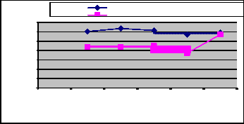
Error of the network

Classical Method

Second derivative method

3500

3000

2500

2000

1500

1000

500

0

Sample1 Sample2 Sample3 Sample4 Sample5

Sample

Table 1: Parameters and their values used in all learning processes

After the segmentation technique as specified by the algorithm the following number of patterns have been obtained for the train- ing

Table 2: Results of Vertical Segmentation Technique

Thus, out of 1000 words sample the 718 words have been cor- rectly segmented and used as the patterns for the training of neu- ral network. The neural network has been trained with conven- tional descent gradient method and from the proposed general- ized second derivative of instantaneous error method with dy- namic mean of the global error. The performance of the network has been analysis. The values of gradient descent and proposed generalized second derivative method are computed for each trail

Figure 4: The Comparison chart for gradient value between

Classical method and generalized second derivative methods

The results in the table 3 are representing the epochs of training
and the presence of error in the network for classical gradient de- scent method and proposed generalized second derivative descent gradient method. The results shown here are the mean of all the trials. The proposed generalized second derivative descent gradi- ent method for the handwritten words recognition is showing the remarkable enhancement in the performance.

5. CONCLUSION:

This paper is following the approach of generalized second de- rivative of instantaneous squared error for its minimization in the weight space corresponds to the presented input-output pattern pairs to exhibit a good generalized behavior to the fed forward neural network for the given training set. The weight modification had consider for the hidden & output layer and inputs & hidden layer, beside this the second derivative of the local errors has ob- tained with respect to both the weights i.e. hidden and output layer. The following observations were made for the entire dis- cussed procedure.
1. The generalized second derivative gradient method gener- ates the minimum of unknown instantaneous error in K- dimensional error surface. The weights have modified for each of this error. These modifications in the weights were obtained with

IJSER © 2013 http://www.ijser.org

International Journal of Scientific & Engineering Research, Volume 4, Issue 8, August-2013 1718

ISSN 2229-5518

the generalized second derivative of this instantaneous square error. The generalized second derivative of the error has obtain with respect to the weights for output layer & hidden layer indi- vidually and also in combination.
2. The proposed method for good generalization is obtaining the point of minimum local error for every input pattern during the training in each step. Once the instantaneous local error mini- mum has obtained, the square mean of this local error minimum with current global error has obtained. This exhibits the current global dynamic error on each step. Further, the weights are again modified with generalized second derivative for the current glob- al error. Thus, the network has trained for the global behavior rather than the individual local behaviors which represent the good generalized behavior of the neural network. This iterative process continues till the global error does not minimize for all the presented input –output pattern pair of training set.
3. The more experiments of complete pattern and analysis are still needed for completely verify the method. The complexity of the algorithm should also analyze and compare with the other methods. These can consider as the extended or future work.

References

[1] A. L. Blum and R. Rivest, “Training a 3- node neural network is

NP-complete”, Neural Networks, (5) 1 (1992) 117-128.

[2] D. R. Hush and B. G. Horne, “progress in supervised neural networks: Whats new since Lipmann”, IEEE Signal Processing magazine, 10 (1993) 8-

39.

[21] Thimm G., Moerland F., and Fiesler E., “ The interchangeability of learning rate an Gain in Back Propagation Neural Netwroks”, Neural Computation 8 (2) (1996) 451-460.

[22] Dhaka V. S. and Singh M. P., “Handwritten character recognition using mod-

ified gradient descent technique of neural networks and representation of

conjugate descent for training patterns”, International Journal of Engineering, IJE Transaction A: Basics, 22 (2) (2009) 145-158

[23] Singh M. P., Kumar S., and Sharma N. K., “Mathematical formulation for the second derivative of backpropagation error with non-liner output function in feedforward networks”, International Journal of Information and Decision Sciences, 2(4) (2010) 352-37

IJSER © 2013

http://www.ijser.org