Inte rnatio nal Jo urnal o f Sc ie ntific & Eng inee ring Re se arc h Vo lume 3, Issue 2, Fe braury -2012 1
ISSN 2229-5518
Finite element analysis of electromagnetic bulging of sheet metals
Ali M. Abdelhafeez, M. M. Nemat-Alla, M. G. El-Sebaie
Material strain hardening models w hich describe mechanical behaviour of the used material at such high speed forming process are of primary importance to get accurate simulation results. Tw o hardening models w ere used in previous researches on this process. But no comparison betw een them w as made to conclude the most accurate model in describing hardening behaviour of the used material.
The current investigations introduce a comparison betw een tw o hardening material models that used in previous researches. The comparison w as made betw een results of numerical simulations and experimental results o btained f rom literature. The used FE model is based on modif ied loose coupling scheme. Simulation results reveal that rate dependant pow er law hardening model gives the most accurate results w ith small average deviation compared w ith experimental data. It reveals also that modif ied loose coupling betw een mechanical and electromagnetic aspects is an eff icient tool f or getting accurate simulation results w ithin short time.
—————————— ——————————
LECTROMAGNETIC forming (EM Forming) process de- pends on generating high intensity transient magnetic fields by forcing high current to flow through a coil posi- tioned very close to the workpiece. When a pulsed high cu r- rent flows through the coil, a transient magnetic field is pro- duced around the coil. This changing field induces eddy cu r- rents in the workpiece opposed in direction with the coil cu r- rent. The eddy currents of the workpiece produce a magnetic field. The magnetic fields of the coil and the workpiece repel each other, producing high repulsive pressure. This pressure is considered as the driving force of deformation. The pulsed high current can be generated by charging capacitor banks at
high voltage and suddenly drain all the charge in the coil.
Because EM forming characterizes by high deformation ve-
locity and no-contact between tool and workpiece, the forming limits of metal sheets can be enhanced [1] in addition to reduc- ing springback and wrinkling [2]. These characteristics drive the researchers to try to benefit from it; especially in the man u- facturing of light weight vehicles body which is fabricated from Aluminium alloys. Because of Aluminium low fracture strain and high springback; EMF is the ideal forming tech- nique to be used for overcoming these drawbacks and benefi t- ing from its high electrical conductivity.
———— ——— ——— ——— ———
M. M. Nemat-Alla, professor of materials science, Assiut University,
Egypt.
M. G. El-Sebaie, professor of metal forming, Assiut University, Egypt.
Several investigations had been done on EM forming in which few were related to electromagnetic sheet metals bul g- ing. One of such early investigations was made by Takatsu et al. [3] in which finite difference modelling and experimental verification was made. Takatsu experimental work considered today as a benchmark in EM bulging of sheet metals . His ex- perimental data had been used by many other previous re- searchers to verify their numerical simulation.
On computing technology advancement, numerical meth- ods began to take increasing role in modelling and simulation of metal forming processes. Fenton and Daehn [4] used a 2D finite difference code to simulate EM forming process with a fully electromagnetic–mechanical coupling. In order to vali- date their computer code the results of the experimental work of Takatsu et al. [3] were used as benchmarks. Steinberg work hardening material model was adopted. Although their mate- rial model ignores strain rate effects, the results showed good agreement with experimental results. This may be a ttributed to the use of material model that has much higher initial yield stress (93 MPa) than the actual value (22 MPa [5]).
El-Azab et al. [6] reported the future needs in modelling EM forming as two major challenges; numerical challenges and material modelling challenges. They claimed that numeri- cal solution of the general fully coupled problem has not been previously achieved. On the other hands the material cha l- lenges are appear in adopting strain rate and temperature de- pendency through the deformation processes. Only their net effects on the deformation process can be observed in labora- tory tests while experimental observation of their effect with time and deformation is difficult due to the high speed of de- formation and biaxiallity of strains.
IJSER © 201 2
Inte rnatio nal Jo urnal o f Sc ie ntific & Eng inee ring Re se arc h Vo lume 3, Issue 2, Fe braury -2012 2
ISSN 2229-5518
Correia et al. [7] made a trial to overcome modelling cha l- lenges of EM forming. They used rate depen dant power law for describing strain hardening behaviour of Takatsu et al. [3] disk material. They considered a simple model of EM bulging process, in which the mechanical and electromagnetic aspects were treated as two independent problems. ABAQUS/Explicit FEM software was used to simulate the deformation of the sheet as explained in Takatsu et al. [3]. The magnetic spatial and temporal pressure distributions were determined using finite difference code which was implemented in ABAQUS user subroutine named VDLOAD to solve magnetic diffusion equations. The obtained pressure was then used as a load to the mechanical problem to calculate the deformation. This coupling technique is known by loose coupling. Although they used strain rate dependent power law, their results are not in good agreement with previous experimental results of Takatsu et al. [3]. This may be due to the consideration of loose coupling scheme without modifications that gives more accurate simulation results as mentioned by Hashimoto et al. [8].
Siddiqui et al. [9] enhanced electromagnetic part of Correia model [7] for getting more accurate simulation results. They compared the obtained simulation results with experimental data [3] and a good agreement was noticed. They concluded that mesh size effects have negligible influence on results due to small thickness size of workpiece.
Recently, Cui et al. [10] simulated experimental work of Takatsu et al. [3] using ANSYS multi-physics FEM software. Strong coupling scheme was used which accounts for ma g- netic pressure change with workpiece deformation . Following Fenton and Daehn [4], the simplified Steinberg Material hard- ening model was used. The simulation results were in good agreement with experimental results but simulation process was time consuming.
Finally from the previous literature survey it can be con-
cluded that two material hardening models were used to de- scribe Takatsu [3] disk material behaviour. These two material hardening models are Steinberg model, and rate dependant power law model. Previous researchers used different FE simulation models that utilized these hardening models and good agreement was obtained. But right comparison between these hardening models must be with the same FE model to conclude the most accurate one.
In this research, an FE model was established based on
modified loose coupling between electromagn etic and me- chanical aspects. This loose coupling strategy was considered before by many other researchers [7], [11], [12], [13]. The model was used to compare these hardening models to de- termine the most accurate one in describing mechanical be- haviour of the used material at these conditions .
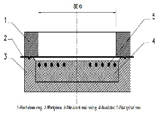
current passes in the coil. Typical process setup is shown in Fig. (1) and dimensions are given in table (1). This setup could be modelled electrically by two mutually coupled circuits that shown in Fig. (2).
TABLE (1)
COIL AND WORKPIECE DIMENSIONS.
Coil | Workpie ce | |||
Major radius | 32 mm | Thickness | 0.5 mm. | |
No. of turns | 5 | Bulged diameter | 80 mm. | |
pitch | 5.5 mm | Overall diameter | 110 mm. | |
Coil/ Workpiece separation distance = 1.6 mm |
Fig. 1. Typical setup of EM bulging of sheet metals.
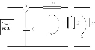
Fig. 2. Electrical model of the process.
Governing differential equations of these magnetically coupled circuits according to Takatsu et al. [3], is:
L d i (t ) d
(M .i
(t )) R .i (t ) 1
i (t )dt 0;
![]()
![]()
1 dt 1 dt
![]()
2 1 1 1
0
(1)
EM sheet metals bulging is a high velocity forming technique in which there is a spiral flat coil positioned near to a flat ci r- cular blank workpiece. A high repulsion pressure produced between coil and workpiece when transient high electrical![]()
![]()
d (L .i (t )) d (M .i (t )) R .i (t ) 0
dt 2 2 dt 1 2 2
With initial conditions:![]()
i (0) 0, i (0) 0, [L d i ] V
1 2 1 dt 1 t 0 0
IJSER © 201 2
Inte rnatio nal Jo urnal o f Sc ie ntific & Eng inee ring Re se arc h Vo lume 3, Issue 2, Fe braury -2012 3
ISSN 2229-5518
Where, L1, L2 are inductance of the coil and workpiece cir- cuit; M is mutual inductance between the two circuits; R1, R2 are electrical resistances of the coil and workpiece circuit; c capacitance of discharge circuit;V0 is initial discharge voltage of the capacitor banks; i1(t) is discharging current as function of time for the coil circuit; i2(t) is induced current function of time for the workpiece circuit.
These two simultaneous equations have the mutual indu c- tance term M which represent the magnetic coupling between the two circuits. The mutual inductance M and the self- inductance of the workpiece L2 change with the workpiece deformation and deformation depends mainly on M and L2. This interdependency makes the mathematical solution of these two equations almos t difficult unless using numerical methods with simplifying assumptions. Assuming that M and L2 are constants and not depend on deformation will simplify this problem. This assumption is part of loose coupling tec h- nique used in tying electromagnetic and mechanical aspects. The equivalent circuit model now could be obtained, and the reduced equation for the current will be [8]:
t
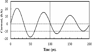
Fig. 3. Variation of electric current i(t) w ith time.
Magnetic pressure generated from magnetic field of the coil current is the driving force of workpiece deformation. Its dis- tribution over the workpiece is not uniform and it is varying
L d i
(t ) R
i (t ) 1
i (t )dt V
(2)
with time and with workpiece deformation. Thus magnetic![]()
c dt
![]()
c c c c 0
c 0
pressure is dependent on workpiece deformation and defor- mation is dependent on applied magnetic pressure. This in-
With initial conditions:![]()
i (0) 0, [L d i ] V
c c dt c t 0 0
Where, Lc is total inductance of the system; Rc is total electri- cal resistance of the system; Cc is total capacitance of the sys- tem; ic(t) is the current passing in the coil; V0 is initial dis- charge voltage of the capacitor banks.
terdependency makes perfect determination of this pressure depends mainly on the electromagnetic-mechanical aspects coupling scheme used.
Assuming magnetic pressure to be independent on work- piece deformation will simplify the analysis with small rela- tive errors in results. Therefore the general magnetic pressure function P(r,t) can be considered as a function of blank radius multiplied by a pressure function of time, i.e.
The solution of Eq. (2) is given by [14]:
P (r ,t ) f
(r ) p (t )
(4)
i (t )
![]()
V 0
Lc
e _ t sin(t )
(3)
The temporal variation of magnetic pressure was expressed before [8] as:
Where,
B (t )2 B
(t )2
(5)
![]()
1
LcC c
( Rc )2
2Lc
p (t ) diff
20
Where, B(t) is magnetic flux density between workpiece
Values of these electrical parameters are given by table (2).
TABLE (2)
and coil; Bdiff (t) is diffused flux density; and µ0 is magnetic permeability of the air.
Magnetic flux density; B(t); is given by [15],
PROCESS ELECT RICAL PARAMET ERS.
B (t ) K 0i (t )
(6)
Where; K is constant depends on workpiece and coil ge- ometry and skin depth.
The diffused magnetic flux can be n eglected for non-
magnetic materials like Aluminium [16], thus;
It can be noticed that the electric current function has an exponentially decayed sinusoidal wave form as shown in Fig. (3).
p (t )
B (t )2
![]()
20
(7)
Consequently from (3), (6) and (7) the final form of tempo-
ral pressure behaviour is![]()
![]()
p (t ) 1 K 2 ( V 0
)2e _ 2 t sin 2 (t )
(8)
IJSER © 201 2
2 Lc
Inte rnatio nal Jo urnal o f Sc ie ntific & Eng inee ring Re se arc h Vo lume 3, Issue 2, Fe braury -2012 4
ISSN 2229-5518
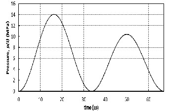
Such variation of temporal behaviour of the magnetic pres- sure is shown in Fig. (4).
The spatial distribution at a given time can be determined by studying the magnetic flux density distribution over the disk radius. This distribution can be found by numerically
simulation package, an implicit dynamic finite element code, which is used in sheet deformation analysis. The dynamic equilibrium equation is given by (9), and the Newmark time integration method is used to solve it [17].
solving Maxwell equations of electromagnetism for specific coil-workpiece geometry. Such numerical solution is beyond![]()
M u C u K u F
(9)
the scope of this research paper.
Previous calculated data [3] of spatial pressure distribution at time of maximum pressure value was used; after normaliz- ing; to determine spatial distribution function. Normalized data was obtained by dividing all pressure values with max i- mum p(t) value and is shown in fig. (5).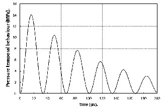
Fig. 4. Te mporal behaviour of magnetic pressure.
Where M represents the mass matrix (Kg), C is the damping
matrix (Kg/s), K is the stiffness matrix (Kg/s2 ), F is load vector
(N). According to Takatsu experimental work [3], workpiece mechanical and electrical properties are listed in table (3).
TABLE (3)
WORKPIECE MATERIAL PROPERT IES
De ns ity | 2750 Kg/m3 |
Young’s Modulus | 80.7 GPa |
Poisson’s ratio | 0.33 |
Yie ld s tress | 22 MPa. |
Ele ctric conductivity | 34.45 MS/ m |
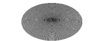
The workpiece is meshed with quadrilateral finite- membrane-strain element with reduced integration points on its surface and 9 integration points through its thickness. Total number of elements is 4000 and the meshed workpiece is shown in fig. (6).
Fig. 6.Non-def ormed w orkpiece mesh.
During deformation, workpiece outer perimeter is consid- ered to be fixed.
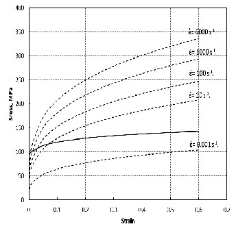
There are two hardening models that are extensively used in modelling JIS A1050-O material which used in Takatsu et al. [3] experimental work. Simplified Steinberg model [4], [10] as given by (10), and rate dependent power law [7], [9] as given by (11).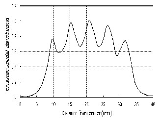
![]()
![]()
93(1 125 )0.1
(10)
![]()
Fig. 5. Pressure spatial distribution over w orkpiece radius.
201
![]()
0.27 0.075
(11)
Now magnetic pressure function has been identified and determined. This function is entered to the mechanical FE model as surface pressure on the bottom surface of the blank with spatial and temporal variation specified before.
The magnetic pressure calculated by (4) is used as bound- ary condition to the structure model and entered to an FEM![]()
![]()
Where is the effective stress in MPa; is the effective strain. These hardening models are shown in fig. (7).
To decide the most accurate model in describing hardening
behaviour of this material; An FE simulation was built which
is based on a modified loose coupling scheme. Next section describes this coupling scheme.
IJSER © 201 2
Inte rnatio nal Jo urnal o f Sc ie ntific & Eng inee ring Re se arc h Vo lume 3, Issue 2, Fe braury -2012 5
ISSN 2229-5518
[3] experimental data. It is clear that the used strain hardening models have a great effect on the simulation results. Obvi- ously, there is a moderate agreement between the experimen- tal results and the rate dependent hardening model simulation results. In addition to a large deviation between the other hardening model simulation results and Takatsu results are clearly appeared.
Fig. 8. Modif ied pressure temporal behaviour.
Fig. 7. Eff ective stress-strain diagrams f or used hardening models (dashed lines represent rate dependent model and solid line represents Steinberg model).
Loose coupling depends on finding the magnetic pressure spatial and temporal distribution independent of workpiece deformation. This is of course untrue and always gives overes- timated simulation results. A modification of this coupling scheme to get more accurate results is mentioned by Hash i- moto et al. [8]. They reported that only the first wave of cur- rent affects deformation of workpiece.
Thus the modified loose coupling scheme considers only the
first wave of current to determine magnetic pressure temporal
behaviour. On the other hand, the spatial pressure distribution function f(r) was specified before from electromagnetic FE simulation. Therefore the total load to be applied on the workpiece surface is P(r,t) = p(t)|modified . f(r), where f(r) is as given by Fig. (5), and p(t)|modified is given by (12) and shown in fig. (8).
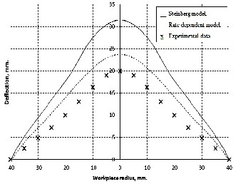
Fig. 9. Final prof ile of def ormed w orkpiece w ith using various hardening models.
1 K 2i (t )2 ,
t
![]()
p t |modified
2 0
0,
t
(12)
The relative errors between simulation results and experi- mental work are calculated over the whole deformed work-
Where, is the periodic time of current wave i(t) and equals 67 µs.
Two runs of the simulation were done each with one of the hardening models previously listed.
The final deformed profile of the workpiece for each harden-
ing model is presented in fig. (9) in conjunction with, Takatsu
piece and presented in Fig. (10). The maximum relative error was about 90 % for Steinberg model while it was about 45 % rate dependent hardening model. It is obvious that the most accurate strain hardening model is rate dependent power law which has a relative error with average value over disk radius of 30 %. This result is logic since the strain rate in this process has very large values and can’t be neglected.
The effective plastic strain distribution on the final d e-
formed disk is shown in Fig. (11). It is clear that a maximum
value of effective plastic strain of 0.45 was achieved at blank
IJSER © 201 2
Inte rnatio nal Jo urnal o f Sc ie ntific & Eng inee ring Re se arc h Vo lume 3, Issue 2, Fe braury -2012 6
ISSN 2229-5518
centre for rate dependent strain hardening model. For the other strain hardening model; the maximum effective plastic strain value was achieved at blank edge which may be not true.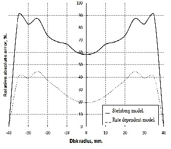
Fig. 10.Re lative absolute error betw een FEM simu lation and experimen- tal data.
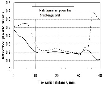
Fig. 11. Ef f ective plastic strain distribution.
Effective plastic strain rate for elements at blank centre and at radial distance of 20 mm are plotted against time as shown in Fig. (12) and (13). It can be noticed that the maximum strain rate over the whole blank attained at centre. The strain rate at blank centre has its maximum value near end of deformation on contrast with strain rate at radial distance 20 mm. This could be explained by the earlier movement of blank outer perimeter than inner perimeters.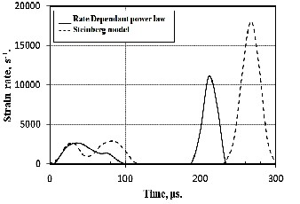
Fig. 12. Eff ective strain rate variation w ith time f or element at blank cen- tre.
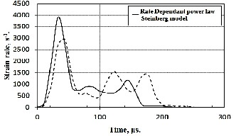
Fig. 13. Eff ective strain rate variation w ith time f or element at 20 mm f rom centre.
In the current investigations a simple and accurate finite element model for the EM forming of sheet metals was intro- duced. Two different strain hardening material models were considered in simulation and the obtained results were com- pared with published experimental data. From the simulation results and comparison between them the following points can be concluded:
1- The introduced simulation model gives simulation re- sults in good agreement with experimental data when used with rate dependent power law hardening model. This is logic since high strain rates were achieved in this process and thus strain rate effects can’t be neglected.
2- The final deformed blank profiles didn’t have any
change in shape for any used strain hardening model but the changes are only in dimensions of the final deformed blank. This means that the final profile depends mainly on the pres- sure spatial and temporal distribution.
3- For rate dependent power law model; maximum values
of strains and strain rates are achieved at blank centre. This
means that failure is possible to occur at centre of the blank.
IJSER © 201 2
Inte rnatio nal Jo urnal o f Sc ie ntific & Eng inee ring Re se arc h Vo lume 3, Issue 2, Fe braury -2012 7
ISSN 2229-5518
[1] Seth, M., Vohnout V. J., Daehn G. S., "Formability Of Steel Sheet In High Ve- locity Impact", J. mater. Process. Tech., 168, pp. 390-400, (2005).
[2] Padmanabhan, M., "Wrinkling And Springback In Electromagnetic
Sheet Metal Forming And Electromagnetic Ring Compression", Mas- ter thesis, The Ohio State University, (1997).
[3] Takatsu, N., Kato, M., Sato, K., Tobe, T., "High Speed Forming Of
Metal Sheets By Electromagnetic Force", J.S.M.E., 31(1), p. 142, (1988). [4] Fenton, G. K., Daehn, G.S., "Modeling Of Electromagnetically
Formed Sheet Metal", J. mater. Process. Tech., 75, pp. 6-16, (1998).
[5] Kondo, K., Suzuki, H. , "Research On The Accuracy Of Sheared Products By Different Working Principles In Precision Shearing", J. mater. Process. Tech., 56, pp. 70-77, (1996).
[6] El-Azab, A., Garnich, M., Kapoor, A., "Modeling Of The Electroma g-
netic Forming Of Sheet Metals: State-Of-The-Art And Future Needs", J Mater. Process. Tech., 142, pp. 744-754, (2003).
[7] Correia, J. P. M., Siddiqui, M.A., Ahzi, S., Belouettar, S., Davies, R., " A Simple Model To Simulate Electromagnetic Sheet Free Bulging Process.", Int. J. Mech. Sci., 50, pp. 1466 -1475, (2008).
[8] Hashimoto, Y., Hideki, H., Miki, S., Hideaki, N. , "Local Deformation
And Buckling Of A Cylindrical Al Tube Under Magnetic Impulsive
Pressure", J Mater. Process. Tech., 85, pp. 209 -212, (1999).
[9] Siddiqui, M. A., Correia, J. P. M., Ahzi, S., Belouettar, S., "A Numeri- cal Model To Simulate Electromagnetic Sheet Metal Forming Proc-
ess.", Int. J. Mater. Form., 1, pp. 1387-1390, (2008).
[10] Cui, X., Mo, J., Xiao, S., Du, E., Zhao, J., "Numerical Simulation Of Elec- tromagnetic Sheet Bulging Based On FEM", Int. J. Adv. Manuf. Tech., pp. 1-8, (2011).
[11] Imbert, J. M., "Increased Formability and the Effects of the
Tool/Sheet Interaction in Elect romagnetic Forming of Aluminum A l- loy Sheet", M.Sc., University of Waterloo, (2005).
[12] Oliveira, D. A., "Electromagnetic Forming of Aluminum Alloy Sheet:
Experiment and Model.", M.Sc., University of Waterloo, (2002).
[13] Pérez, I., Aranguren, I, González, B, Eguia, I, "Electromagnetic Form- ing: A New Coupling Method", Int. J. Mater. Form., 2, pp. 637-640, (2009).
[14] Xu, W., Fang, H., Xu, W., "Analysis Of The Variation Regularity Of The Parameters Of The Discharge Circuit With The Distance Between Workpiece And Inductor For Electromagnetic Forming Processes ", J. mater. Process. Tech., 203, pp. 216-220, (2008).
[15] Zhang, H., Murata, M., Suzuki, H., "Effects Of Various Working
Conditions On Tube Bulging By Electromagnetic Forming", Journal of Materials Processing Technology, 48, pp. 113-121, (1995).
[16] Kleiner, M., Beerwald, C., Homberg, W., "Analysis of Process P a-
rameters and Forming Mechanisms within the Electromagnetic
Forming Process", Annals of the CIRP, 54, pp. 225 -228, (2005).
[17] Yu, H. P., Li, C.F., Deng, J.H. , "Sequential Coupling Simulation For Electromagnetic Mechanical Tube Compression By Finite Element Analysis", J. Mater. Process. Tech., 209, pp. 707-713, (2009).
IJSER © 201 2