International Journal of Scientific & Engineering Research, Volume 4, Issue 12, December-2013 454

ISSN 2229-5518

Faster Convex Hull Computation By Reducing Computatinal Overhead and Time

Ngangbam Herojit Singh , Laiphrakpam Dolendro Singh

Abstract — Finding the convex hull of a point set has applications in research fields as well as industrial tools. This paper presents a pre-processing algorithm for computing convex hull vertices in a 2D spatial point set. Based on the position of extreme points we divide the exterior points into four groups bounded by rectangles (p-Rect). Then inside each p-Rect we recursively find and check the extreme points to verify if they are eligible to be convex hull points or not. The process gives a small set of candidate points for convex hull computation. Efficiency of the algorithm is evaluated with respect to time and space. Performance comparison with other classical algorithms shows that implementation of this pre- processing algorithm significantly improves their performance by reducing computational overhead and time.

Index Terms — Quick Convex Hull, Recursion, p-Rect, Point rotation, Preprocessing Algorithm.

1 INTODUCTION

——————————  ——————————
Normally, the final convex hull contains only a few points,
The convex hull (CH) of a set Q of points is the smallest convex polygon P for which each point in Q is either on the boundary of P or in its interior [1]. Its application area includes computer visualization, ray tracing, path finding, visual pattern matching, verification methods and geometry. It is also used as a tool to construct geometric shapes, the GIS applications such as area cut, subdivision of Triangulated Irregular Network (TIN) and DTM generation and area dynamic calculation [2].
Convex hull algorithms are broadly divided into two
categories: 1) graph traversal and 2) incremental [3]. The graph traversal algorithms construct CHs by identifying some initial vertices of CH and later finding the remaining points and edges by traversing it in some order. The Graham scan [4], Jarvis march [5] and Monotone chain [6] are such algorithms. Incremental algorithms first find an initial CH and then insert or merge the remaining points, edges or even sub CHs as they are discovered, into current CH sequentially or recursively to obtain the final CH. Quickhull [7] and Divide-and-Conquer [8] belong to this class.
Most of these algorithms scan and process all the points
one by one resulting in much computational overhead.
and most of the points are in the interior of convex hull. Based on this concept we devised a fast preprocessing algorithm which filters out most of the non-convex hull points. The final CH points can be easily found out of the candidate points discovered after the pre-processing, using any classical algorithm with minimal overhead.

1.1 RELATED WORKS

Recently, several novel algorithms are developed to obtain CH for a point set. Fu and Lu in [2] propose an improved algorithm which finds convex hull boundary by recursively dividing the set of points into sub regions and updating them after each recursive division. A polynomial- time algorithm for the D-convex hull of a finite point set in the Plane is discussed in [10]. Some algorithms enhance performance though excluding non-convex hull vertexes to reduce the analysis of the minimum convex hull, such as grouping the set of points [9, 11], establishing the auxiliary grid field [12] and obtaining the extreme points as in the quick convex hull [7, 13, 14, 15]. The Floyd quadrilateral method and octagonal methods are some of the quick convex hull algorithms. Huang and Liu [16] present an algorithm

International Journal of Scientific & Engineering Research, Volume 4, Issue 12, December-2013 455

ISSN 2229-5518

based on binary tree that builds convex hull with scattered point based on the concept of quick convex hull.
Clarkson, Mulzer and Seshadhri developed a self- improving algorithm to compute planar convex hull points [17]. Liu and Wang [18] propose a reliable and effective CH algorithm based on a technique named Principle Component Analysis for pre-processing the planar point set. A fast CH algorithm with maximum inscribed circle affine transformation is described in [19]. Some algorithms are designed targeted toward harnessing the power of GPUs as in [20].

1.2 PROPOSED ALGORITHM

Our algorithm is based on the fact that in a given set of randomly scattered points, over a two dimensional Euclidean space, only the points to the exterior of the region covered by the point set, participate in constructing the convex hull. Rests of the interior points are not of any importance. So we try to obtain the exterior points near the boundary and check whether they are proper candidates for being convex hull
points.

PBL_Ymin is the point with minimum y-coordinate.

The points in Bottom-Right (BR) region are bounded by a

p-Rect whose two opposite corner points are PBR_Xmax and

PBR_Ymin , where

PBR_Xmax is the point with maximum x-coordinate.

PBR_Ymin is the point with minimum y-coordinate.

The points in Top-Left (TL) region are bounded by a p-
Rect whose two opposite corner points are P TL_Xmin and

PTL_Ymax , where

PTL_Xmin is the point with minimum x-coordinate.

PTL_Ymax is the point with maximum y-coordinate.

The points in Top-Right (TR) region are bounded by a p-
Rect whose two opposite corner points are PTR_Xmax and

PTR_Ymax , where

PTR_Xmax is the point with maximum x-coordinate.

PTR_Ymax is the point with maximum y-coordinate.

In case of a conflict between two or more points having
same extreme x-coordinate or y-coordinate, we resolve that using the following rules.
If number of points having minimum x-coordinate is greater than 1 then, for Bottom-Left p-Rect we take the point with minimum y-coordinate and make it PBL_Xmin . While for

IJSER

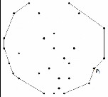
For this purpose we divide the point set into four
rectangular region or p-Rects (see Fig. 1). The four p-Rects are
called Bottom-Left (BL), Bottom-Right (BR), Top-Left (TL) and Top-Right (TR). The points inside the p-Rects are called points of interest. The four p-Rects distribute the entire point set into
5 different clusters based on location of individual points
(location based clustering). Each of the clusters contains some
edges of the convex hull. Each of the four p-Rects is constructed by two corner points which have extreme x/y coordinates chosen as explained next.

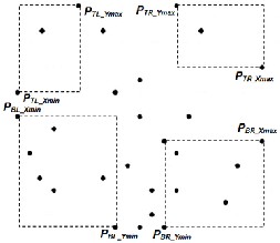
Fig. 1.Four regions (p-Rect) with the points of interest constructed by their two corner points

The points in Bottom-Left (BL) region are bounded by a p- Rect whose two opposite corner points are P BL_Xmin and PBL_Ymin , where

PBL_Xmin is the point with minimum x-coordinate.

Top-Left p-Rect we take the point with maximum y-
coordinate and make it PTL_Xmin .
If more than one point has maximum x-coordinate then, for Bottom-Right p-Rect we take the point with minimum y- coordinate and make it PBR_Xmax . While for Top-Right p-Rect the point with maximum y-coordinate is chosen as PTR_Xmax .
If number of points having minimum y-coordinate is
greater than 1 then, for Bottom-Left p-Rect we take the point with minimum x-coordinate and make it PBL_Ymin and for Bottom-Right p-Rect we take the point with maximum x- coordinate and make it PBR_Ymin .
If more than one point has maximum y-coordinate then,
for Top-Left p-Rect we take the point with minimum x- coordinate and make it PTL_Ymax . While for Top-Right p-Rect we take the point with maximum x-coordinate and make it PTR_Ymax .
The above 8 points are directly included in the convex hull candidate point set. There may be less than 8 points in case two extreme points are coincident. For example, PBL_Xmin and PTL_Xmin can be the same point if there is only one point with minimum x-coordinate.
The points which have the minimum/maximum x- coordinates or y-coordinates but do not belong to any of the four p-Rects are directly included in the convex hull candidate point set because of the obvious fact that points with extreme x/y coordinate are definitely part of convex hull. These points are identified from the cluster which does not belong to any of the four p-Rects. The number of candidate points detected

International Journal of Scientific & Engineering Research, Volume 4, Issue 12, December-2013 456

ISSN 2229-5518

from this cluster is proportional to the size of the cluster and distribution of points over the two dimensional Euclidean space.

A. Processing the Points of Interest

Points inside the p-Rects go through a recursive process which gradually finds out the boundary points in that region. But before explaining the process we present a brief description of a related concept, which determines the clockwise/anti-clockwise orientation of a point with respect to another point.

Let p0 (x0 , y0 ), p1 (x1 , y1 ) and p2 (x2 , y2 ) are three discrete points and we want to determine whether p2 is clockwise or anticlockwise from p1 with respect to p0 . For that we calculate cross product between the directed segments p0 p1 and p0 p2 like in (1) [1].

(p2 - p0 ) × (p1 - p0 ) = (x2 - x0 )(y1 - y0 ) - (x1 - x0 )(y2 - y0 ) (1)
If the sign of this cross product is negative, then p2 is counter-clockwise with respect to p1 . A positive cross product
• If none of them are clockwise from PBL_Ymin then we leave further processing.
• If only any one of them is clockwise from PBL_Ymin then we include it to the convex hull point set and terminate further processing in this section.
• If both of them are clockwise from P BL_Ymin or collinear
then we construct a smaller p-Rect keeping P′BL_Xmin and

P′BL_Ymin as corner points and recursively process the points

of interest in the new Bottom-Left (BL') p-Rect using above
steps in search of new convex hull points.

(a) (b)

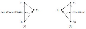
indicates a clockwise orientation (see Fig. 2). A cross product of 0 means that the points p0 , p1 , and p2 are collinear.

(c)

(d)

Fig. 2. Using cross product to determine point orientation. (a) Negative cross product means counter clockwise rotation. (b) Positive cross product indicates clockwise rotation.

1) Bottom-Left p-Rect Operation: For this section the points of interest is the set of points {p1 , p2 , p3 ...} where each pi = (xi , yi ) such that

PBL_Xmin .x < xi < PBL_Ymin .x

PBL_Ymin .y < yi < PBL_Xmin .y

Out of this set we find out P′ BL_Xmin and P′BL_Ymin the same way we found PBL_Xmin and PBL_Ymin for the outer Bottom-Left p- Rect. Further processing depends upon the following 3 cases.
Case 1: If there are no such points then we terminate
further processing in this p-Rect.
Case 2: If both are same point then we check whether the
point is clockwise or anticlockwise from point P BL_Ymin with respect to point PBL_Xmin (see Fig. 3). If it is clockwise or collinear then we include it to the convex hull candidate point set and terminate further processing.
Case 3: If both are different than we check whether they
are clockwise or anticlockwise from point PBL_Ymin with respect to point PBL_Xmin . Again we will have 3 scenarios:

Fig. 3. Operation on the Bottom-Left p-Rect points. (a) Checking orientation of P′BL_Xmin and P′ BL_Ymin from PBL_Ymin . (b) Creation of new Bottom-Left (BL′) p-Rect and processing points inside. (c) Inclusion of new candidate points inside inner p-Rect. (d) Inclusion of points collinear with P BL_Ymin .

2) Bottom-Right p-Rect Operation: For this section the points of interest is the set of points {p1 , p2 , p3 ...} where each pi = (xi , yi ) such that

PBR_Ymin .x < xi < PBR_Xmax .x

PBR_Ymin .y < yi < PBR_Xmax .y

From this set we find out P′BR_Xmax and P′BR_Ymin the same way we found PBR_Xmax and PBR_Ymin for outer Bottom-Right p- Rect. Further processing based on these two points is done using similar 3 cases explained in Bottom-Left p-Rect operation.
Here the points are checked whether they are clockwise or anticlockwise from point PBR_Xmax with respect to point PBR_Ymin (see Fig. 4).
The recursive operation continues until no new candidate points are found for convex hull.

International Journal of Scientific & Engineering Research, Volume 4, Issue 12, December-2013 457

ISSN 2229-5518

3) Top-Right p-Rect Operation: For this section the points of interest is the set of points {p1 , p2 , p3 ...} where each pi = (xi , yi ) such that

PTR_Ymax .x < xi < PTR_Xmax .x

From this set we find out P′ TL_Xmin and P′TL_Ymax the same way we found PTL_Xmin and PTL_Ymax for outer Top-Left p-Rect. Further processing based on these two points is done using similar 3 cases explained in Bottom-Left section operation.
Here the points are checked whether they are clockwise or

PTR_Xmax .y < yi < PTR_Ymax .y

anticlockwise from point P
(see Fig. 6).

TL_Xmin

with respect to point P

TL_Ymax

Out of this set we find out P′TR_Xmax and P′TR_Ymax the same way we found PTR_Xmax and PTR_Ymax for the outer Top-Right section. Further processing based on these two points is done using 3 cases similar to the cases explained in Bottom-Left p- Rect operation.
The recursive operation continues until no new points are found eligible for convex hull point set.

B. Removing the non-convex hull points

After performing the four sectional operations the points we get are called candidate points for convex hull. We call them candidate points because there are some extraneous points which do not actually belong to the convex hull. Figure
7(a) shows such a point PS . To remove such points we perform standard convex hull algorithms such as Graham's scan or Jarvis's March on the obtained candidate point set (see Figure 7(b)).

(a) (b)

Fig. 4. Bottom-Right p-Rect operation of the points. (a) Checking orientation of P′BR_Xmax and P′BR_Ymin from P BR_Xmax . (b) Processing of points inside new Bottom-Right (BR′) section.

Here the points are checked whether they are clockwise or
anticlockwise from point PTR_Ymax with respect to point PTR_Xmax
(see Fig. 5).

Fig. 5. Top-Right p-Rect operation of the points. Here both P′ TR_Xmax and

P′TR_Ymax are same and it is anticlockwise from P TR_Ymax .

The recursive operation continues until no new points are found eligible for convex hull point set.

4) Top-Left p-Rect Operation: For this section the points of interest is the set of points {p1 , p2 , p3 ...} where each pi = (xi , yi ) such that

PTL_Xmin .x < xi < PTL_Ymax .x

PTL_Xmin .y < yi < PTL_Ymax .y

(a) (b)

Fig. 6. Operation of the Top-Left p-Rect points. (a) Checking orientation of P′TL_Xmin / P′TL_Ymax from P TL_Xmin . (b) Inclusion of the point & termination of search in this section.

(a) (b)

Fig. 7. Removal of non-convex hull point. (a) PS is a non-convex point. (b)

PS removed after applying Graham’s scan.

2 Algorithm Analysis

A. Time Efficiency Analysis

Our algorithm contains four recursive point region operation each of which finds the candidate points for convex hull and hence its running time can be described using a

International Journal of Scientific & Engineering Research, Volume 4, Issue 12, December-2013 458

ISSN 2229-5518

recurrence equation or recurrence. Moreover these four operations are symmetric. So if we find the time complexity of
any of the four operations avoiding multiplication to the constant factor 4, that will be time complexity of the entire algorithm.
It is basically a divide-and-conquer algorithm in which the divide operation includes searching the points of interest in a specific region. Combine step includes searching for points with minimum and/or maximum x and/or y coordinates, checking their rotation and keeping the distinct candidate points in a storage (e.g. stack) for further processing by standard convex hull algorithms. In conquer step we recursively solve a sub problem of 1/b the size of original input point set. The value of b can be anything depending upon orientation of the points, without affecting the final time complexity.
For the two search operations if we apply linear search it requires O(n) time on n points. O(1) time is required for both rotation checking and storing the candidate points. So the entire combine step takes O(n) time as shown in (2).

C(n) = O(n) + 2.O(1) = O(n) (2)

algorithm, then the total running time T(n) = T'(n) + T(m) will be less than that of the convex hull algorithm applied on non
preprocessed point set.

B. Space Efficiency Analysis

This divide-and-conquer is not much space efficient, as in each recursive call we rest and store them separately for further processing. As a result in each recursive call a new memory space of size (1/b)th of the memory space of previous step is reserved.

C. Test of Numeral Value

We developed a simulation of our proposed algorithm using C programming language and tested it over several configurations of scattered points. We are presenting the test results in the following tables. The Graham's scan algorithm implementation uses merge sort, while Jarvis's march uses linear search for finding the next pivot point.
In Tab.1. shows a particular case of processing 10,000 points
for Bottom-Left section. As we can see after each level of recursion, number of points of interest reduces quickly with great speed of convergence. This condition also holds for
other larger amount of point set. In fact in our simulations we
IJSEfound very fewRcases when the process reached 4th level of
Running time for Divide step is

D(n) = O(n) (3) So the recurrence for the worst-case running time T(n) of the

algorithm is:
recursion.
Since
O(1) if n ≤ 3

T(n)= �T �n� + O(n) if n > 3 (4)

C(n) + D(n) = O(n) + O(n) = O(n) (5)

Solution to this recurrence is T(n) = O(n lg n). As we can see the prime factor affecting the time complexity of the preprocessing algorithm is the time required by the point searching operation. As we are applying a linear search in our algorithm, its time complexity is not dependent on the randomness and the entropy of the 2-D point set. If we apply a more efficient searching algorithm such as binary tree search running time can be reduced to O(lg n lg n).
Let after the preprocessing step we get m candidate points,
where m << n and n is very large. So for processing by standard convex hull algorithms like Graham's scan (O(n lg n)) and Jarvis's march (O(nh), h is the number of points in convex hull), the required time will be quite less, O(m lg m) and O(mh) respectively.

Tab. 1. Statistics of Point Reduction after Each Level of Recursion.

In Tab. 2. gives a comparative running time (in ms) analysis by several algorithms under our test environment. It is very clear that with the growing number of input points the efficiency of our algorithm gets better. The preprocessing algorithm narrows down the amount of candidate points to such an extent that the applied Graham's scan or Jarvis's march completes very quickly.
Hence if T'(n) is the running time of our preprocessing algorithm and T(m) is the running time of any convex hull

International Journal of Scientific & Engineering Research, Volume 4, Issue 12, December-2013 459

ISSN 2229-5518

REFERENCES

Tab.2. Performance Comparision with other Algorithms(MS).

In Tab. 3. we present a comparative study of average performance gain over the classical Graham scan and Jarvis march algorithms by some of the recent convex hull algorithms presented in [16][21][22]. All these algorithms use almost similar principle for convex hull computation and the performance gain is computed based on the computation time required by them. The study shows that in most of the cases our proposed algorithm gives the highest performance gain.

[1] Thomas H.Cormen, Charles E.Leiserson, Ronald L.Rivest,

Introduction to Algorithm, 3rd Edition, MIT press, Cambridge, pp

1014-1047, 2009.

[2] Zhongliang Fu and Yuefeng Lu, “An efficient algorithm for the convex hull of planner scattered point set,” International Archives of the Photogrammetry, Remote Sensing and Spatial Information Sciences, XXII ISPRS Congress, Melbourne, Australia, pp. 63-66, 2012.

[3] D. Avis, D. Bremner and R. Seidel, “How good are convex hull algorithms?,” in Computational Geometry, vol. 7, pp. 265-301, 1997.

[4] R. L. Graham, “An efficient algorithm for determining the convex hull of a finite planar set,” in Information Processing Letters, vol. 1, pp.

132-133, 1972.

[5] R. Jarvis, “On the identification of the convex hull of a finite set of points in the plane,” in Information Processing Letters, vol. 2, pp. 18-

21, 1973.

[6] A. M. Andrew, “Another efficient algorithm for convex hulls in two dimensions,” in Information Processing Letters, vol. 9, pp. 216-219,

1979.

[7] C. B. Barber, D. P. Dobkin and H. Huhdanpaa, “The Quickhull algorithm for convex hulls,” Acm Transactions on Mathematical Software, vol. 22, pp. 469-483, Dec 1996.

[8] F. P. Preparata and S. J. Hong, “Convex hulls of finite sets of points

in two and three dimensions,” in Communications of the ACM, vol. 20, pp. 87-93, 1977.

[9] Wang Jiechen, “Study of optimizing method for algorithm of minimum convex closure building for 2D spatial data,” Acta Geodaetica et Cartographica Sinica, 31(01), pp. 82-86, 2002.

[10] V. Frank and J. Matouek, “Computing D-convex hulls in the plane,”

Computational Geometry, vol. 42, pp. 81-89, 2009.

[11] Zhang Zhongwu and Wu Xincai, “Algorithm for convex hull of planar massive scattered point set,” in Computer Engineering, 35(09), pp. 43-45, 48, 2009.

Tab. 3. Comparision of Performance Gain.

3 CONCLUSION

In this paper we have discussed about a preprocessing algorithm for finding convex hull points, which is based on the fact that only the points existing to the boundary of a region covered by a randomly scattered set of points, take part in constituting the convex-hull. We have discussed about its running time complexity and also proved through real- time simulation results that this preprocessing improves the overall running time of convex hull algorithms. Although the purpose of developing this algorithm was to find all valid convex hull points and use it as a standard Quick Convex Hull algorithm. But as we saw that the algorithm outputs some invalid convex hull points too and removing them was not possible, keeping the running time constraint into consideration. So, we decided to keep it as a preprocessing step. Our future work will be focusing on how we can remove this deficiency and also reduce the space complexity so that it can be used as a standalone convex hull algorithm.

[12] Wang Jiechen and Chen Yanming, “A gird-aided algorithm for determining the minimum convex hull of planar points set,” in Geomatics and Information Science of Wuhan University, 35(04), pp. 403-

406, 2010.

[13] Yu Xiangyu, Sun Hong, Yu Zhixiong, “An improved algorithm to determine the convex hull of 2D points set,” in Journal of Wuhan University of Technology, 27(10), pp. 81-83, 92, 2005.

[14] Wu Wenzhou, Li Lifan and Wang Jiechen, “An improved Graham algorithm for determining the convex hull of planar points set,” in Science of Surveying and Mapping, 35(06), pp. 123- 125, 2010.

[15] Cheng Sanyou and Li Yingjie, “A new algorithm of minimum convex hull and its Application,” in Geography and Geo-Information Science, 25(05), pp. 43-45, 2009.

[16] Linna Huang and Guangzhong Liu, “Proved Quick Convex Hull Algorithm for Scattered Points,” in International Conference on Computer Science and Information Processing (CSIP), pp. 1365-1368,

2012.

[17] K. L. Clarkson, W. Mulzer, and C. Seshadhri, “Self-improving algorithms for convex hulls,” in Proc. SODA, pp. 1546-1565, 2010.

[18] B. Liu and T. Wang, “An effcient convex hull algorithm for planar point set based on recursive method,” in Acta Automatica Sinica, vol.

38, pp. 1375-1379, 2012.

[19] R. Liu, B. Fang, Y. Y. Tang, J. Wen and J. Qian, “A fast convex hull algorithm with maximum inscribed circle affine transformation,” Neurocomputing, vol. 77, pp. 212-221, 2012.

International Journal of Scientific & Engineering Research, Volume 4, Issue 12, December-2013 460

ISSN 2229-5518

[20] A. Stein, E. Geva, and J. El-Sana, “CudaHull: Fast parallel 3D convex hull on the GPU,” Computers & Graphics, vol. 36, pp. 265-271, 2012.

[21] Gang Mei, John C.Tipper and Nengxiong Xu,” An Algorithm for Finding Convex Hulls of Planar Point Sets,” in 2nd International Conference on Computer Science and Network Technology (ICCSNT), pp.

888-891, 2012.

[22] Min Zhou, Bo Yang, Yun Liang, Qiong Huang and Junzhou Wan, “Fast Algorithm for Convex Hull of Planer Point Set,” in Information

& Computational Science, vol. 10, No. 4, pp. 1237-1243, 2013.

————————————————

Ngangbam Herojit Singh was born in Imphal West, Manipur,India. He received his M.Tech. from Anna University Chennai in 2013.Currently,he is working as Research Assistant in National Institute of Technology,Manipur. His research interests NetworksSecurity,Algorithms, Pattern Recognitio .(Email ID:herojitng@gmail.com).

Laiphrakpam Dolendro Singh was born in Imphal East, Manipur,India. He received his B.E. from Anna University Chennai in 2011.Currently,he is pursuing M.E from National Institute of Technology,Agartala. His research interests include Networking,Image processing.(Email ID:doltana@gmail.com).

IJSER