International Journal of Scientific & Engineering Research, Volume 4, Issue 7, July-2013 2236
ISSN 2229-5518
Fast RC Circuit Simulation Using Artificial Neural
Networks
Mohamed G. Kamal, Mohamed S. El-Mahallawy , Mohamed W. Fakhr , Yasser Y. Hanafy
Index Terms— Model Order Reduction, RC trees, Cicrcuit modeling, Artificial Neural Netwoks, Mean square error
—————————— ——————————
odel Order Reduction (MOR) methods are used to model the input–output behavior of any large scale dy- namical system over a certain range of operation using significantly smaller dimension matrices [1–2]. Simulation of large scale circuits requires solving of a high order differential equation at each node in the circuit which is time consuming, numerically demanding and heavily CPU intensive especially for very large scale circuits. So, searching for a reduced order model which preserves the dominant characteristics of the full order model and reduces the analysis time will be a demand- ing solution for this problem. The role of this reduced order model is to preserve the dominant characteristics of the sys- tem response of the model and reduces the simulation time and CPU usage[3]. Moreover, MOR offers an excellent route to computing the input–output response eliminating a large number of features that do not have a significant influence on
the system output.
In order to obtain a reduced order model, retain the critical
frequencies and minimize the mean square error, several
methods of MOR have been introduced. Each of these meth-
ods has its advantages and disadvantages. Moreover, There is
no method that gives the best results for all of the systems.
Therefore, each system uses the best method with respect to its
application. Now, some of these methods are introduced be-
low.
Several Methods have been introduced to obtain the de
————————————————
• Mohamed SaadEl Mahallawy is currently an assciate professor in electronics
and Communications engineering at Arab Academy For Science and Technol-
sired reduced order model. In Seventies, the Pade approxima- tion method was introduced [4]. BaniHani and De [5] compa- red some Model order reduction methods for fast simulation
of soft tissue response using the point collocation- based method of finite spheres. G. Parmar et al. [6] presented a mod- el order reduction using genetic algorithm for unit impulse input and measured the integral square error and impulse response energy. C.B. Vishwakarma and R. Prasad [7] pro- posed a method that approximates the numerator polynomials using Pade approximation and approximates the denominator polynomials using some clustering techniques, this method ensures the stability of the system. Alsmadi et al. [8] proposed a method for MOR of dynamical systems based on Artificial Neural Networks (ANN) transformation along with the linear matrix ine-
quality (LMI) optimization method. Alsmadi et al. [3] proposed a method for model order reduction using substructure preser- vation.
In this paper, a new technique for modeling any RC Tree circuit using ANN is presented based on minimizing the mean square error referred as cost function.
The rest of the paper is organized as follows. Section 2 in- troduces the transfer function representing the reduced model. In section 3, the training process of the artificial neural net- work is illustrated. In section 4, the results are introduced and finally in section 5, the conclusion is presented.
The discrete time system representing any RC circuit is de- scribed by the following transfer function:
𝑘−1
ogy, Egypt. E-mail: mahallawy@ieee.org![]()
![]()
𝐺(𝑠) = 𝑌(𝑠) = 𝑎𝑜+𝑎1 𝑠+𝑎2 𝑠+⋯+𝑎𝑘−1 𝑠
(1)
• Yasser Y. Hanafy is currently the president's assistant for information at
𝑋(𝑠)
𝑏𝑜 +𝑏1 𝑠+𝑏2 𝑠2 +⋯+𝑏𝑘𝑠𝑘
Arab Academy For Science And Technology, Egypt. E-mail:yhanafy@vt.edu
where 𝑎𝑖 represents the numerator coefficients, 𝑏𝑖 R represents
the denominator and k is the number of coefficients, X(s) is the
input and Y(s) is the output of the system.
The corresponding transfer function of the reduced model
IJSER © 2013 http://www.ijser.org
International Journal of Scientific & Engineering Research, Volume 4, Issue 7, July-2013 2237
ISSN 2229-5518
which contains the dominant poles only is written as:
where 𝑤 is the weight that connects the i'th th
node and the current
node , 𝑥𝑖 is the output from i'
node of the previous layer, b is the
𝐺𝑟 (𝑠) =
𝑌 (𝑠)
𝑋(𝑠)
![]()
= 𝑐𝑜+𝑐1 𝑠+𝑐2 𝑠2 +⋯+𝑐𝑛−1 𝑠𝑛−1
𝑑𝑜 +𝑑1 𝑠+𝑑2 𝑠2 +⋯+𝑑𝑛𝑠𝑛
(2)
threshold value of the current node and f is the activation function.
The outputs of the hidden layers are distributed over the next layer until the last one where the outputs are fed into a layer of output
where 𝑐𝑖 R represents the numerator coefficients, 𝑑𝑖 represents
the denominator coefficients and n is the number of the re-
duced coefficients.
To obtain a stable macro-model, the reduced model trans-
fer function is converted to the pole residue model using par-
tial fraction expansion and can be written as:
units.
In this paper, The ANN is trained to estimate the dominant poles and residues of any high order transfer function regardless to the values of the poles and residues of the impulse or step response representing the transfer function
The learning process is performed using The back- propagation algorithm which adjusts the free parameters
𝑛 𝑅𝑖
![]()
𝐺𝑟 (𝑠) = ∑𝑖=0 𝑠−𝑃 (3)
(weights and biases) of the network to minimize the mean
square error (MSE) referred as the cost function [3]as written
below:
where R are the residues and P are the poles of the reduced
𝑀𝑀𝑀 = 1 ∑𝑁
1 ∑ (𝑦 (𝑛) − 𝑧 (𝑛))2
model.![]()
![]()
𝑁 𝑛=1 2
𝑗∈𝐶 𝑗 𝑗
(6)
Hence, the impulse response equation of the reduced order model can be written as:
− 𝑡
where 𝑀𝑀𝑀 is the cost function as a measure of learning per- formance, 𝑦𝑗 (𝑛) is the desired response of the full order model,
𝑧 (𝑛) is the output response of the reduced model, neuron 𝑗 is![]()
𝑔𝑟 (𝑡) = ∑𝑛
𝑅𝑖 𝑒
𝑃𝑖
(4)
𝑗
the output node, set C includes all the neurons in the output
To construct a reduced model whose impulse response is very close to the original model in an efficient and fast way regardless to the full model size, an ANN is trained to esti- mate the impulse response of the RC Tree circuit and minimiz- ing the mean square error between the impulse response curves of the full order model and reduced order model [3].
In order to model any circuit, two approaches are uesd
; the physical approach and the black box approach. Each of
these approaches has its advantages and disadvantages. How-
ever, when there is no complete knowledge of the physical
parameters of a device the black box approach is used. The
behavior of the circuit is captured by using a set of input data
and the corresponding output response data. Then an approx- imation is performed over a set of measured data in order to find a convenient analytical equation to use it in the simula- tion of the circuit. The main advantage of the black box ap-
proach is that the simulation time is small compared to the physical approach.
layer of the network and N is the total number of patterns con- tained in the training set.
Considering an RC tree circuit that contains a large num- ber of poles and residues, the ANN is used to reduce its order to the second order. The ANN is offline trained with the im- pulse response curves of circuits with different values of poles and residues and used online to estimate the values of the two dominant poles and residues of the reduced transfer function.
The Artificial Neural Network used contains two hidden layers and one output layer with an activation function which is tangent hyperbolic sigmoid in the hidden layers and purelinear in the output layer.
The network is trained using gradient descent algorithm with 22000 data points with a mean square error (cost func- tion). The range of the dominant poles used is between 0 and
0.4 while the range of the residues of the dominant poles is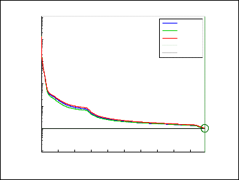
between 0.5 and 1.
Best Validation Performance is 1.0178e-06 at epoch 1968
Multilayer perceptron NN is one of the most common 10-1
types of NN used in the simulation of non linear functions. It
is used to implement nonlinear transformations for function 10-2
approximations[9]. The network is composed of a set of source
nodes that represent the input layer, one or more hidden lay- -3
10
ers and an output layer. Each layer computes the activation
function of the weighted sum of the inputs. The input signal -4
10
propagates through the layers in a forward direction from the
input layer to the output layer (and passes through all of the
Train Validation Test
Best
Goal
hidden layers layer by layer)[10].The input-output relation- 10
ship between of each node of the hidden layer is as fol-
-6
lows[11]: 10
𝑦 = 𝑓(∑𝑖 𝑤𝑖 𝑥𝑖 + 𝑏) (5)
-7
10
0 200 400 600 800 1000 1200 1400 1600 1800
1968 Epochs
IJSER © 2013 http://www.ijser.org
International Journal of Scientific & Engineering Research, Volume 4, Issue 7, July-2013 2238
ISSN 2229-5518
Figure 1 shows the training process of the ANN. In this fig ure, the mean square error between the exact (SPICE simulat ed) and the estimated (using ANN) is 1.0178*10-6 after training the ANN for 1968 epochs.
After completing the training process, the Neural Network is tested in 4 different cases using generated testing data other than that of the training data.
In the first case, we consider 22000 different test patterns of
8th order RC tree circuits; each pattern contains two dominant
poles and 6 non-dominant poles. The trained ANN is used to
estimate the dominant poles and residues of each pattern. The
It is clear that the ANN is able to estimate the dominant poles and residues of the full order model with an acceptable range of error.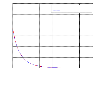
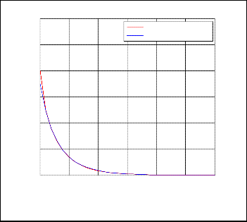
Figure 4 shows an example of the exact and estimated im- pulse response of the tested patterns of the RC circuit trees of order 8 with 2 dominant poles and 6 non-dominant poles. The ANN succeeded to estimate the impulse response with mean square error of 4.1065*10-4 which is acceptable.
3
exact impulse response estimated impulse response
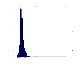
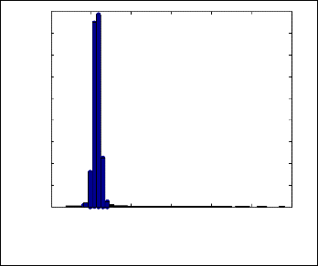
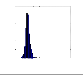
trained network succeeded to reduce the order of the transfer
function of the circuit to the second order with mean square
error and mean absolute error histograms shown in figures 2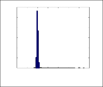
and 3.
2.5
2
12000
1.5
1
10000
8000
0.5
6000
4000
0
0 0.5 1 1.5 2 2.5 3
Time[s]
Fig. 4. Impulse response of the 8'th order RC Tree (1'st case).
2000
0
3 3.5 4 4.5 5 5.5 6 6.5
In the second testing case, we consider another 22000 pat- terns of 10th order RC tree circuits impulse responses; each pattern contains two dominant poles and 8 non-dominant
Mean Square Error
Fig. 2. Mean square error histogram (1'st case)
-4
x 10
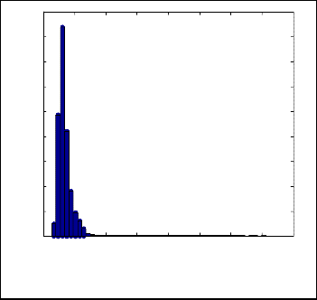
poles, the same trained ANN is used to estimate the dominant poles and residues of each pattern. The trained network suc- ceeded to reduce the order of the transfer function to the se- cond order with mean square error and mean absolute error histograms shown in figures 5 and 6.
8000
9000
7000
8000
6000
7000
5000
6000
4000
3000
5000
4000
3000
2000
2000
1000
1000
0
3 4 5 6 7 8 9 10 11
0
2.05 2.1 2.15 2.2 2.25 2.3 2.35
Mean Absolute Error
Fig. 3. Mean absolute error histogram (1'st case).
-3
x 10
Mean Square Error
Fig. 5. Mean square error histogram (2'nd case).
-3
x 10
IJSER © 2013 http://www.ijser.org
International Journal of Scientific & Engineering Research, Volume 4, Issue 7, July-2013 2239
ISSN 2229-5518
9000
8000
7000
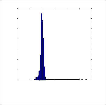
dues of each pattern. The trained network succeeded to reduce the order of the transfer function to the second order with mean square error and mean absolute error histograms shown in figures 8 and 9.
6000
7000
5000
6000
4000
3000
5000
2000
4000
1000
3000
0
0.008 0.009 0.01 0.011 0.012 0.013 0.014 0.015 0.016
Mean Absolute Error
Fig. 6. Mean absolute error histogram (2'nd case).
2000
1000
Figures 5 and 6 show that the ANN is still able to estimate the dominant poles and residues of the full order models and the error is approximately still the same after increasing the number of the non-dominant poles and residues
Figure 7 shows the impulse response of the tested pattern of an RC tree circuit of order 10 with the same 2 dominant poles used previously and 8 non-dominant poles. The ANN is able to estimate the impulse response with mean square error
0.0021 which is increased compared to example 1 as the num- ber of non-dominant poles is increased but acceptable.
0
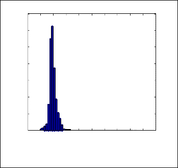
Fig. 8. Mean square error histogram (3'rd case).
7000
6000
3
2.5
exact impulse response
estimated impulse response
5000
4000
2 3000
1.5
2000
1000
1
0.5
0
0.01 0.011 0.012 0.013 0.014 0.015 0.016 0.017 0.018 0.019 0.02
Mean Absolute Error
0
0 0.5 1 1.5 2 2.5 3
Time[s]
Fig. 9. Mean absolute error histogram (3'rd
case).
Fig. 7. Impulse response of the 10'th order RC Tree (2'nd case).
In case 3, we consider another 22000 different patterns of an 12'th order RC tree circuits impulse responses, each pattern contains two dominant poles and 10 non-dominant poles. The same ANN is used to estimate the dominant poles and resi-
It is clear that the ANN is still able to estimate the dominant poles and residues of the full order model and the error is greater than that of the previous cases but still acceptable.
Figure 10 shows the impulse response of a tested pattern of an RC tree circuit of order 12 with 2dominant poles and 10 non-dominant poles. The ANN succeeded to estimate the im- pulse response with mean square error 0.0031 with more error
IJSER © 2013 http://www.ijser.org
International Journal of Scientific & Engineering Research, Volume 4, Issue 7, July-2013 2240
ISSN 2229-5518
than that of examples 1 and 2 but still acceptable.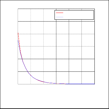
6000
3
2.5
exact impulse response
estimated impulse response
5000
4000
2 3000
1.5
2000
1000
1
0.5
0
0.034 0.035 0.036 0.037 0.038 0.039 0.04 0.041 0.042 0.043
Mean Absolute Error
0
0 0.5 1 1.5 2 2.5 3
Time[s]
Fig. 12. Mean absolute error histogram (4'th case).
It is clear that the ANN is still able to estimate the domi-
Fig. 10. Impulse response of the 12th
order RC tree (3'rd
case)
nant poles and residues of the full order model and the error is increased compared to the previous cases due to the effect of the large number of the non-dominant poles and residues.
Figure 13 shows the impulse response of a tested pattern of
In the last case, another 22000 pattern of 20'th order RC tree circuit is tested; each pattern contains two dominant poles and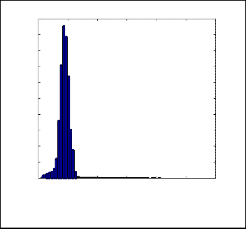
18 non-dominant poles. The same ANN is used to estimate the dominant poles and residues of each pattern. The trained net- work succeeded to reduce the order of the transfer function to the second order with mean square error and mean absolute error histograms shown in figures 11 and 12.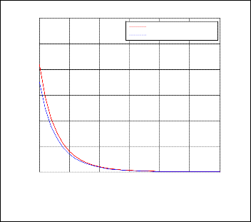
RC tree circuit of order 20 with 2 dominant poles and 18 non- dominant poles. The ANN succeeded to estimate the impulse response with mean square error 0.0069 which is large com- pared to the previous examples as the number of poles and residues is increased.
3
5000
2.5
exact impulse response
estimated impulse response
4500
2
4000
3500
3000
2500
1.5
1
2000
1500
0.5
1000
500
0
0 0.5 1 1.5 2 2.5 3
Time[s]
0
6.5 7 7.5 8 8.5 9 9.5
Fig. 13. Impulse response of the 20'th order RC Tree (4'th case).
Mean Square Error
th
-3
x 10
A comparison between the values of the exact and estimat-
Fig. 11. Mean square error histogram (4'
case)
ed dominant poles (P1, P2) and residues (R1, R2) for all the examples mentioned previously is given in table 1.
TABLE 1
IJSER © 2013 http://www.ijser.org
International Journal of Scientific & Engineering Research, Volume 4, Issue 7, July-2013 2241
ISSN 2229-5518
Exact and estimated dominant poles and residues of 8'th, 10'th
,12'thand 20'th order RC circuit with the same dominant poles.
[10] S. Geva, J. Sitte, "A constructive method for multivariate function approximation by multilayer perceptrons", IEEE Trans. Neural Net- works 3, pp. 621–624, 1992.
[11] S. Haykin, Neural Networks: A Comprehensive Foundation, Mac-
millan College Publishing Company, New York, 1994.
A new technique is developed to estimate the poles and residues of the reduced order model of any system (transfer func- tion representing an RC circuit) regardless to the number of poles and residues representing the RC circuit using Artificial Neural networks. This technique is obtained by training the ANN with the impulse response curves of different RC circuits to obtain a model. This model estimates the dominant characteristics of the full order model without using nodal analysis equations used by the simulation programs (e.g. SPICE) and retains them in the reduced order model that produces a very close response com- pared to the full order model. This technique will reduce simula- tion time with an acceptable accuracy compared to SPICE pro- gram.
[1] Antoulas, Athanasios C. ''Approximation of large-scale dynamical systems,'' Society for Industrial and Applied Mathematics, vol. 6,
2009
[2] Rudnyi, Evgenii B., and Jan G. Korvink. "Review: Automatic Model Reduction for Transient Simulation of MEMS-based Devices," Sensors Update 11.1, pp. 3-33, 2002
[3] Othman M.K. Alsmadi, Zaer. S. Abo-Hammour, Adnan M. Al- Smadi, "Artificial neural network for discrete model order reduction with substructure preservation,” Applied Mathematical Modelling vol. 35 no. 9, pp. 4620–4629, 2011.
[4] Y. Shamash, Stable reduced order models using Pade' type approxi- mation, IEEE Lett. AC-19, pp.615–616, 1974.
[5] S.M. BaniHani, S. De, "A comparison of some model order reduction
methods for fast simulation of soft tissue response using the point collocation-based method of finite spheres," Eng. Comput., vol. 25, no. 1, pp. 37–47, 2009.
[6] G. Parmar, M.K. Pandey, V. Kumar, "System order reduction using GA for unit impulse input and a comparative study using ISE & IRE," International Conference on Advances in Computing, Commu- nication and Control, pp. 3–7, 2009.
[7] C.B. Vishwakarma, R. Prasad, "Clustering method for reducing order
of linear system using Pade approximation," IETE J. Res., vol. 54. no.5, pp. 326–330, 2008.
[8] Othman M.K. Alsmadi, Zaer. S. Abo-Hammour, and Adnan M. Al-
Smadi, "Efficient Substructure Preserving MOR Using Real-Time Temporal Supervised Neural Network," NDT 2010, Part II, CCIS 88, pp. 193–202, 2010.
[9] M. Avci, "Neural network-based design approach for submicron
MOS integrated circuits," Mathematics and Computers in Simulation
79.4, pp. 1126-1136, 2008.
IJSER © 2013 http://www.ijser.org