By the methodology and results of [7] the emissions to make a delivery with a distance and a given flow can be calculated by the generic formula below:
International Journal of Scientific & Engineering Research, Volume 5, Issue 9, September-2014 70
ISSN 2229-5518
Evolutionary Algorithm for the Bi-Objective Green
Vehicle Routing Problem
El Bouzekri El Idrissi Adiba, El Hilali Alaoui Ahemd
Abstract— The amount of pollution emitted by a vehicle depends on many factors such as the total distance travelled and its load. In this paper, we present and define the bi-objective Green Vehicle Routing Problem (bi- GVRP) in the context of sustainable transportation. The bi- GVRP is the problem of finding routes for vehicles to serve a set of customers while minimizing the total travelled distance and the total emissions of dioxide of carbon (CO 2 ). We apply the genetic algorithm to solve bi- GVRP benchmarks and perform statistical analysis to evaluate and validate obtained results. The algorithm shows obtains good results and proves the explicit interest grant to emission emitted by vehicle and total distance minimization objective.
—————————— ——————————
he important role of logistics management, in recent decades, geared to rapidly grow in various activities and helps to optimize the existing production and distribution processes; this includes several internal factors like technology, globalization and competition. However the transportation system is an essential key in a logistics chain, where the cost of transport may be one-third of the cost of logistics [1]. The objective of the logistics process is to optimize transportation related costs like travelled distance, time, routes flexibility and reliability. Moreover current trends in fuel consumption and CO2 emitted, these are projected to increase by nearly 50% by 2030 and by 80% by 2050 (Cars and trucks represent about 75% worldwide in fuel consumption of CO2 emitted of road transport) [2]. For these reasons, transportation companies and governments start taking explicitly into account emissions reduction objectives in the definition of their working plans. Then, the generated working plans must minimize both cost and CO2 emissions. These two objectives are not necessarily positively correlated and for some cases they are completely conflicting. The basic transportation model generally used to represent the problem of finding routes for vehicles to serve a set of customers is the Vehicle Routing Problem (VRP) [3]. The scope of this paper is the study and the definition of the bi-objective Green Vehicle Routing Problem (bi- GVRP). The bi-VRP was defined to
represent a class of multi-objective optimization problems.
The bi- GVRP asks for designs vehicle routes to serve a set of
customers while minimizing the total travelled distance and
the total CO2 emissions with respect to classical routing constraints, mainly capacity constraints. Consequently, we
implement a genetic algorithm (GA) to solve the bi-GVRP
————————————————
• El bouzekri el idrissi Adiba is PHD student in Modelling and Scientific
Computing Laboratory, Department of Mathematics, Faculty of Fez. B. P.
2202 Route of Imouzzer Fez Morocco
E-mail: b.i.adiba1@gmail.com
• El Hilali Alaoui Ahmed is PHD in Modelling and Scientific Computing
Laboratory, Department of Mathematics, Faculty of Fez. B. P. 2202 Route of Imouzzer Fez Morocco mail: elhilali_fstf2002@ yahoo.fr
model, with an aggregation method that solves non-convex and non-smooth multi-objective optimization problems. In the next section, we present the concept of green transportation, enumerate all emission factors and how CO2 emissions could be estimated and then integrated into quantitative models. Section 3 define the bi-objective green vehicle routing problem (bi-GVRP), review the corresponding literature and, propose a mathematical model for the bi-GVRP. In section 4 present the evolutionary solving approach based on the GA. Section 5 reports the GA implementation details and computational results. Finally, conclusions of this project are presented and some perspectives for future work are stated.
Transportation sector comprise the everyday carrier of millions of tons of freight and numbers of passengers and despite its importance to the world life, it is one of the great contributors to existing pollutant particles in the air, particularly carbon dioxide (CO2 ). The global CO2 emissions from the transportation sector have grown by 45% from 1990 to 2007, and are expected to continue to grow by approximately 40% from 2007 to 2030 [1]. So, Bjorklund [4] defines “Green Transportation” as a: “Transportation service that has a lesser or reduced negative impact on human health and the natural environment when compared with competing transportation services that serve the same purpose”. Recently, the concept of green transportation for sustainable development has soared due to governmental regulations and customers preference for green products. Consequently, transportation companies are reviewing their processes to take into account such concern. In some cases, transforming the traditional logistics systems to be environmentally friendly shall even lower the costs enabling it to meet classic logistics objectives. Moreover, the green transportation system could be completed by determining emission factors and quantifying trucks emissions to integrate them into the logistics systems networks.
IJSER © 2014 http://www.ijser.org
International Journal of Scientific & Engineering Research, Volume 5, Issue 9, September-2014 71
ISSN 2229-5518
specific policy objectives.
The mode of road transport in this paper refers to transport by Heavy Duty Vehicle (HDV) only (32–40 ton for general merchandise). According to the emissions function for the HDV truck given by [5] and [6] some assumptions are made:
• the average speed is 80km/h;
• the gradient of a road is not taken into account in general the truck considered here is fully loaded with
25000 Kg weight.
By the methodology and results of [7] the emissions to make a delivery with a distance and a given flow can be calculated by the generic formula below:![]()
E(q, d) = d × [( efl − eel )q + e ]
(3)
Where:
Q el
• E(q,d) = the CO2 emissions from a vehicle in kg/km with the variable of load q in ton and d in Km;
• efl = the CO2 emissions of a fully loaded (by weight)
vehicle, (efl = 1.096 kg/km for HDV truck);
• eel = the CO2 emissions of an empty vehicle, (eel=
0.772 kg/km for HDV truck)
• Q = the volume capacity of a vehicle.
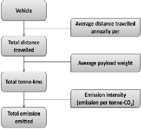
Fig 1. Relationships and variables affecting freight transport emission emitted
Total emission emitted per tonne CO2 depends on the number of vehicles, the average distance they travel, and the extent to which they are loaded. It is difficult to do an exact estimation because of the uncertain effects on climate change and the setting of a price tag on human health.
When an engine is started below its normal operating
Typically, distance, time, and cost are the parameters used to produce, respectively, a matrix of distance, time, and cost between all delivery points and depot. Now, the objective is to design routes that generate the lowest levels of CO2 emissions to atmosphere and, in order to achieve this goal, it is necessary to build a matrix of CO2 emissions based on the estimation of CO2 emitted between each link [8]. The linearization of flow and emissions for the arc ij can be displayed as the emissions matrix:
e − e
temperature, it uses fuel inefficiently, and the amount of
Eij (q, d) = dij × (
fl el
Q
)qij + eel
(4)
pollution produced is higher than when it is hot. These observations lead to the first basic relationship used in the calculation method [6]:
In this section, it is shown how to estimate CO2 emissions from transport freight. Thereafter, we incorporate those
concepts in to the methodology used to solve the vehicle
Where:
E = E hot + Estart + Eevaporative
(1)
routing problem.
• E = the total emission
• Ehot = the emission produced when the engine is hot
• Estart = the emission produced when the engine is cold
• Eevaporative = the emission produced by evaporation
(only for VOC : Volatile Organic Compound)
Indeed, we assume that the underlying transport level supply networks are often over long distances; which Eevaporative implies in neglecting emissions at the vehicle start. Then CO2 are not affected by the term. Consequently, formula (1) can be simplified and detailed as this for CO2 emissions:
The goal that CVRP (Capacity Vehicule Routing Problem) aims at is minimizing total travelling kilometres, and total assigned vehicles, to satisfy green transportation requirements by reducing consumption level and consequently reducing the CO2 emissions from road transportation. Seemingly, the awareness of the contribution of CVRP to green transportation was initiated with the studies of [2] and [8]. However, regarding the existing literature they argue that reduction in total distance will in itself provide environmental benefits due
E = Ehot
(2)
to the reduction in fuel consumed and the consequent
IJSER © 2014 http://www.ijser.org
International Journal of Scientific & Engineering Research, Volume 5, Issue 9, September-2014 72
ISSN 2229-5518
pollutants. Palmer [8], on the other hand, suggests an integration of logistical and environmental aspects into one freight demand model with the aim of enhancing policy analysis. Citing the most relevant and explicit paper ones to the considerations of green transportation we may start by mentioning the introduction of the “Pollution Routing Problem (PRP)” by [9]. They develop PRP as an extension of the classical VRP with a broader and more comprehensive objective function that accounts not only the travel distance, but also the amount of greenhouse emissions, fuel, travel times and their costs. ElBouzekri, in [7] and [10], regards emission matrix as a load dependent function, and add it to
the classical CVRP to extend traditional studies on CVRP with the objective of minimizing emission vehicle emission. For solving these models they use the hybrid ant colony and genetic algorithm for its resolution. All these studies have been published recently; this shows that the topic is at its very beginning. The objective of our work is to find routing and transportation policies that give the best compromise between travelling costs and CO2 emissions. In this paper, we consider emissions minimization as a separate major objective in addition to distance minimization. Therefore, we define a multi-objective combinatorial optimization problem named the bi-objective green vehicle routing problem (bi-GVRP).
All the works cited above have been focusing on in minimizing the cost, the number of used resources, or maximizing the gain. In this section we present the difference in decisions made by CVRP and GVRP. Assuming there are three customers served by one vehicle departing and returning at depot denoted by 0. Our parameters are: efl =
1.096 kg/km for HDV truck; eel= 0.772 kg/km for HDV truck and Q= 25000 kg is the volume capacity of a vehicle. Demands and locations of the customers/depots are shown in Table 1.
,
TABLE 1.
DATA USED IN THE EXAMPLE
ID | Coordinate | Demand | |
Depot | 0 | (1,1) | 0 |
Customer 1 | 1 | (2,3) | 10000 |
Customer 2 | 2 | (4,2) | 7000 |
Customer 3 | 3 | (5,5) | 8000 |
IJSER © 2014 http://www.ijser.org
International Journal of Scientific & Engineering Research, Volume 5, Issue 9, September-2014 73
ISSN 2229-5518
TABLE 2
DISTANCE AND EMISSION TOTAL OF THE EXAMPLE (a)
Route in Fig. 2(a) | |||
i, j | dij | Qij | Eij |
(0,1) | 2,236 | 25000 | 2,450 |
(1,2) | 2,236 | 15000 | 2,160 |
(2,3) | 3,162 | 8000 | 2,768 |
(3,0) | 5,657 | 0 | 4,367 |
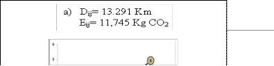
Dij = 13.291 Km, Eij =11,745 Kg CO2 |
TABLE3
DISTANCE AND EMISSION TOTAL OF THE EXAMPLE (b)
Route in Fig. 2(b) | |||
i, j | dij | Qij | Eij |
(0,1) | 2.236 | 25000 | 2,450 |
(1,3) | 3.606 | 15000 | 3,484 |
(3,2) | 3.162 | 7000 | 2,728 |
(2,0) | 3.162 | 0 | 2,441 |
Dij= 12.166 Km, Eij=11,104 Kg CO2 |
TABLE 4
DISTANCE AND EMISSION TOTAL OF THE EXAMPLE (c)
• known fleet size;
• homogeneous fleet (trucks loading 25,000 Kg);
• single depot;
• deterministic demand;
• oriented network;
Denote by V= {0,1…n} a set of n nodes, each representing a vehicle destination. The nodes are numbered 0 to n, node 0 being the depot and nodes 1 to n the delivery points. The transportation process will be carried by a set Z= {0,1…m} of m vehicles. For presenting the integer linear programming model for VRP, the variables below are introduced:
• si: service time of the node i;
• Q : capacity of vehicle;
• cij : cost of vehicle between the nodes i and j;
• Di: the demand of node i, where node i represents a single customer;
• dij : distance between the nodes i and j;
• tij : driving time between the nodes i and j;
• T k : maximum allowable driving time for vehicle k;
The decision variables are:
• qij : the amount charged to the vehicle k between nodes i and j
1 if vehicle k drives from customer i to customer j
• xk =
It is not difficult to find the shortest total distance in Figure 2
(b)(0-1-3-2-0) or 0-2-3-1-0 in Figure.2(a), where these two
routes have identical distances of 12.166. However, these
routes are different in terms of emission emitted [(a) is
Eij=11.580 (b) is 11.104]. Moreover, we can find in the route (c):
0-1-2-3-0 with a higher emission emitted of 11.745 and a longer
distance of 13.291(Table 2, Table 3, Table 4). The best solution is found with (b) because the vehicle first serves the customers with the larger demands and the shortest distance so that emissions can be lowered later in the route after the heavier goods have been unloaded. This example shows that there is a need to develop a new optimization algorithm with lower emissions and shortest distance as objectives to optimize.
ij
0 otherwise
k 1 if vehicle k visits customer i
• yi =
0 otherwise
We consider two different objectives:
• Minimize the cost of transport
• Minimize the level of vehicle emissions
The relative cost of transport can be expressed by:
n n m
f : ∑∑∑ cij . xij
(1)
The solution for the BI-GVRP determines a set of delivery routes that satisfies the requirements of distribution points and obtains the minimum travelled costs and the minimum volume of emitted CO2 while visiting each customer once and with respect to vehicles capacity constraints. It is clear that the BI-GVRP is an NP-hard problem due to the fact that it is an extension of the standard VRP; this problem exhibits the
i = 0 j= 0 k =1
For any arc {i,j} in the route, where point j is the next point the vehicle serves after it leaves point i, the cost for travelling from i to j can be expressed as cij = c0 × dij , where c0 is the unit fuel cost, dij is the distance from i to j. The function of emission emitted by the vehicle is:
following characteristics:
n n m
![]()
fl el k k
(2)
g : ∑∑∑ dij
Q
q ij + eel xij
i = 0 j= 0 k =1
Our objective function is composed by two different objectives and they are not on the same scale, which is why we used the
IJSER © 2014 http://www.ijser.org
International Journal of Scientific & Engineering Research, Volume 5, Issue 9, September-2014 74
ISSN 2229-5518
aggregation method for to transform the bi-objective problem (PBO) into a problem (PBOλ ) which combines the various functions of the problem into a single objective function; so the
problem is to minimize:
Constraints (11) indicate the reduced cargo of the vehicle after a customer visit and equaling the demand of the customer, which also prohibits any illegal sub-tours
n k n k (11)
![]()
Min
f
g
(3)
∑ qij − ∑ q ji =
j= 0 j= 0
Di ,
∀ i = 1, ..., n
β
![]()
+ β
i ≠ j i ≠ j
f
2
Where βi reflects the relative importance of the objectives and
Constraint (12) does not permit that any vehicle exceed the maximum allowable driving time per day T k :
determining the values of
β1 and
β2 is a political décision.
n n n
This research further assumes that the two objectives have
∑∑ t ij xij +
∑ si yi ≤ Tk , ∀ k = 1, ......, m , i ≠ j
(12)
different weights (β1 = 60%) . Thus
f * and g* is the best
i =1 j=1 i =1
Finally, we introduce constraint (13) to avoid sub tours:
values founded in the first phase where the problem is mono-
objective.
∑∑ xk ≤ ![]() S
S ![]() − 1 ;
− 1 ;
i∈S i∈S
j≠ i
![]()
![]()
∀ k = 1,......, m ; S ⊂ {1.....n}, 2 ≤ S ≤ n (13)
The delivery process must satisfy fleet capacity constraints (Qk ) and maximum allowable driving time (Tk ) . Our goal will be to minimizing the sum of the total vehicle emissions emitted and the total cost of transport. We distinguish three types of constraints in our problem: the routing constraints, capacity constraints and schedule constraints.
Constraints (4), (5), (6) and (7) ensure that each vehicle tour begins and ends at the depot:
n
This work seeks to explore some of the potential of artificial evolutionary techniques, in particular genetic algorithms (GAs) [11], [12], for optimization and search in control systems engineering. In this work, multi-objective optimization weighted linear aggregation has been used with genetic algorithms in a single-objective fashion, like conventional optimizers. Nevertheless, the main goal is to maintain a population which is a set of solutions (called in this context individuals), through a fixed number of iterations. A numerical value called fitness, depending on the function
objective of the corresponding. At each iteration, a number of
∑
i = 0
x0i ≤
1 , ∀ k = 1, ..., m ( 4)
individuals are selected according to their fitness in order to
n
k
i0 i = 0
≤ 1,
∀ k = 1, ..., m ( 5)
create new ones by applying two operators: Crossover and
Mutation. At the end of the iteration, a replacement phase is
n n
∑ y k
≤ M.∑ x k , ∀k ∈ {1, 2 , ..., m} (6)
applied to select the individuals which pass to the next
i 0j
i = 1 j = 1
n n
iteration.
∑ y k
≤ M.∑ x k ,
∀k ∈ {1, 2 , ..., m}(7 )
The Genetic algorithm is organized as follows:
i j0
i = 1 j = 1
Constraint (8) guarantees that each node, except the depot, is visited by a single vehicle:
n
1. Coding the solutions
2. Generating the initial population
3. Repeating
• Selection
∑
k =1
yi ≤
1, ∀ i = 1, ..., m
(8)
• Crossover
• Mutation
Furthermore, constraints (9) assure that each node, except the
depot, is linked only with a pair of nodes, one preceding it and the other following it. When a vehicle k arrives to a location, it has to pull through, which respect the law of Kirtchof
n n
• Replacement
Until a stoping condition
∑ x ji =
∑ xij
, ∀ k = 1, ..., m , ∀ i = 1, ..., n (9)
For solving BI-GVRP with GAs, each vehicle identifier (gene
j=1 j=1
Constraint (10) ensures that no vehicle can be over loaded, while constraint (11) limits the maximal load carried by the
vehicle and forces qk to zero when x k = 0 ;
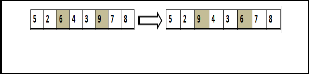
with index 0) represents in the chromosome a separator between two different routes, and a string of customer identifiers represents the sequence of deliveries that a vehicle must cover during its route. Figure 4 shows a representation of a possible solution with 10 customers and 4 vehicles. Each
route begins and ends at the depot.
ij ij
n n
q k ≤
Q xk ,
∀ k = 1, ..., m
(10)
∑∑
i = 0 j=1
i ≠ j
ij ij
IJSER © 2014 http://www.ijser.org
International Journal of Scientific & Engineering Research, Volume 5, Issue 9, September-2014 75
ISSN 2229-5518
Fig. 3: Typical representation of each chromosome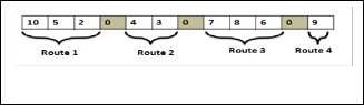
An initial population is built such that each individual must at least be a feasible candidate solution, i.e., every route in the initial population must be feasible and initialized randomly.
Evaluate the fitness of each chromosome in the population is evaluated. The fitness function is the inverse of the total distance. The lower the total distance, the higher fitness it is likely to have.
The calculated fitness helps now to select members for the next generation. We use in our work the selection type roulette. A selection of roulette is an operator in which the chance of a chromosome getting selected is proportional to its fitness (or rank). This is where the concept of survival of the fittest comes into play.
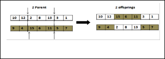
The “crossover” is a genetic operator that combines two chromosomes (parents) to produce a new chromosome (children). The idea behind crossover is that the new chromosome may be better than both of the parents if it takes the best characteristics from each of the parents. Crossover occurs during evolution according to a user definable crossover probability.
The elitism strategy keeps a small number of good individuals and replaces the worst individuals in the next generation without going through the usual genetic operations.
Genetic parameters are population size, number of generations, crossover rate, and mutation rate from existing studies. In addition, the genetic parameters also include a selection operator which randomly selects a chromosome from the population. It is hard to find the best parametric values, so the following genetic parameters were applied through repeated experiments (Table 5).
Table 5. Genetic parameters
This section describes computational experiments carried out to investigate the performance of the proposed GA. The algorithm was coded in C++ and run on a PC with 1.6 GHz CPU and 512 MB memory. In order to check the efficiency of the improved GA, this study analyzed the results of the existing examples by using the Eilon Data [14] and Fisher Problem [15]. Table 6 shows the results of the existing problems using our GA and the average total travel distance obtained over 5 runs. A comparison of the solution quality in terms of minimizing travel distances is done considering our approach with respect to other metaheuristics proposed previously in literature. These metaheuristics are GA proposed in [15] and HGA proposed in [16].
Fig. 4: Figure 5: Example of 2-point crossover
The other genetic operator is “mutation”, which is applied to a single solution with a certain probability. Mutation operator makes small random changes in the solution. These random changes will gradually add some new characteristics to the population, which could not be supplied by the crossover. In the study, partial-mapped crossover (PMX) and swap mutation [13] are used for genetic operations of permutation based chromosomes, (figure 6).
Fig. 6: Example of mutation
IJSER © 2014 http://www.ijser.org
International Journal of Scientific & Engineering Research, Volume 5, Issue 9, September-2014 76
ISSN 2229-5518
The symbol “----” means that the corresponding problem is
Table.6
Comparison of experimental results for different heuristics and GA on VRP
not tested or that a feasible solution cannot be obtained following the literature. For this purpose, we need to compare our results with those of previous works. The comparison includes one objective: minimization of the routing cost over the feasible ones. The proposed algorithm has shown to be competitive with the best existing methods in terms of solution quality, where our approach is better than hybrid AG except for the instances E-n22-k4 and E-n33-k4, while problem, E-n45-k4, gaves the same distance of 724. However, searching the bests solution in term of cost can slow down the algorithm. Our GA needs some refinements especially for the local search algorithm to speed up its execution. Finally, the results obtained in Table 6 by our genetic algorithm are effective and show the viability to generate very good quality solutions for the CVRP.
Now, to evaluate our approach to solve BI-GVRP problem, which minimize both CO2 emissions and total distance related to freight transport, we tested its performance on a set of instances randomly generated from 10 to 100 requests. In these instances, there is a depot point, which coordinate is (0, 0), a set of customer points, with coordinate randomly chosen in the region [0 Km, 100 Km], and an unlimited homogenous fleet of vehicles, where the capacity of a vehicles is 25,000 kg. The load volumes of customers randomly belong to the value range [500
Kg, 2500 Kg], and the service time of customers is fixed at 15 minutes. We also suppose that the service period of a vehicle belongs to the time window [08 h, 18 h], and we fixed the average speed of vehicles at 80 km/h. The Table 7 shows the best results found by mono-objective function to minimize the CO2 emissions and minimize the total distance, where n is the number of customers; the columns TE, TD, TD* and NV show the total emissions evaluated following the GVRP algorithm, the corresponding total distance, the total distance evaluated with CVRP algorithm and the number of vehicles respectively for the best solution found.
In the following for solving the BI-GVRP, we are consider the
f* and g* presented in Table 7 (TE , TD* respectively). Our main
Table. 7
Results obtained for 10 different instances of 10 to 130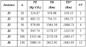
requests
goal being to minimize the total emissions, the weight of the emission function ((α=60%) is higher than the cost function, and the results are presented in Table 8.
These two objectives may be positively correlated with each other, or they may be conflicting with each other. In other
Table. 8
words, the routing cost of a solution increases as the number of vehicles increase. This behavior is hardly to be determined by the classical approach (weighted sum approach or using single objective) while it is easily analyzed by the suggested approach. Remark that these alternate Pareto solutions are clearly comparable and the decision maker can decide which the best solution based on his/her preferences. In instance I6, the routing cost is steadily decreased from 358.53 to 358.07 which indicate the conflicting behaviour between the two objectives. Moreover, in most of instances according to Table 6, just a single Pareto solution is reported that is the best solution generated by the suggested GA method. While conventional single-objective vehicle routing approaches are unable to explore the conflicting behaviour of objectives, the GA algorithm is adequate to easily discover the behaviour for a multi-objectives vehicle routing problem. But when the costs of vehicle counts and minimum travelling distance for reducing the emissions are important, the MOP approach can be effective and generates a set of equally valid BI-GVRP solutions as non-dominated solutions. These solutions represent a range of possible solutions, from which the decision maker (DM) to decide which is preferable. According to Table 8, the results obtained by the suggested model are quite good as compared to the best published results and the average GA performance is sufficient with respect to
IJSER © 2014 http://www.ijser.org
International Journal of Scientific & Engineering Research, Volume 5, Issue 9, September-2014 77
ISSN 2229-5518
time and quality.
This paper suggested a new model and solution for multi- objective green vehicle routing problem (BI-GVRP) using goal programming and genetic algorithms. This paper considered the BI-GVRP as a multi-objective problem where total vehicles emissions and total travelling distance are minimized. By the same token this idea the decision maker specifies optimistic aspiration levels for the objective functions of the problem and deviations from these aspiration levels were minimized. Nevertheless, BI-GVRP is known to be NP-Hard, thus, the proposed mathematical model cannot be solved in a polynomial time to find the best solution of the problem. An efficient genetic algorithm was suggested for solving BI-GVRP formulation that incorporates the concept of Pareto’s optimality for the multi-objective optimization. The proposed genetic algorithm use a string of customer identifiers which represent the sequence of deliveries that a vehicle must cover during its route and each vehicle identifier represented a separator between two different routes in the chromosome. Was applied to explore a larger area of solution space as well. At the end, the algorithm was applied to solve the 6 instance GVRP proposed by ElBouzekri et al.[7], [10]. According to the produced results, the suggested approach was quite sufficient as compared to the best published results and the average GA performance was adequate.
[1] ITF. “Reducing transport greenhouse gas emissions: Trends & Data. Leipzig, Germany“ Bakground for the 2010 International Transport Forum, 2010
[2] A Sbihi. and R WilliamEglese.: “The relationship between vehicle routing and scheduling and green logistics a literature survey“ Lancester: Lancaster University Management School Working Paper, 2007/027
[3] P. Toth, , D. Vigo, “The Vehicle Routing Problem“ SIAM, Philadelphia ISBN
0898715792, (2001)
[4] M.Bjorklund, “Influence from the business environment on environmental purchasing — Drivers and hinders of purchasing green transportation services“Journal of Purchasing & Supply Management 17, 2011: 11–22.
[5] H, Hassel, J. Samaras, “ Methodology for calculating transport emissions and energy consumption (Report for the Projet MEET) “ Transport Research Laboratory. Edinburgh (1999).
[6] J. Jancovici,.; “Bilan Carbones: Calcul des Facteurs D’émissions et Sources
Bibliographiques Utilisées“ ADEME, Paris, France. 2007
[7] A.Elbouzekri, , M. Elhassania, & A. El Hilali Alaoui. A hybrid ant colony system for green capacitated vehicle routing problem in sustainbale transport. Journal of Theoretical & Applied Information Technology, 53(2), (2013).
[8] A. Palmer “The Development of an Integrated Routing and Carbon Dioxide Emissions Model for Goods Vehicles (PhD thesis)",School of Management. Cranfield University.Cranfield, UK (2007)
[9] B. Tolga, G. Laporte. "The Pollution-Routing Problem." Transportation Research
Part B, 2011
[10] A. El Bouzekri, A. El Hilali Alaoui, Y. Benadada “A Genetic Algorithm for Optimizing the Amount of Emissions of Greenhouse GAZ for Capacitated Vehicle Routing Problem in Green Transportation“. International Journal of Soft Computing, 8: 406-415. 2013
[11] J.H.. Holland “Adaptation in Natural and Artificial Systems “University of
Michigan Press. Ann Arbor, Michigan; re-issued by MIT Press (1992).
[12] D.E, Goldberg, “Genetic Algorithms in Search, Optimization, and Machine
Learning, Addison-Wesley, New York“ 1989.
[13] M. Gendreau., Hertz A., Laporte G.: “A Tabu Search Heuristic for the
Vehicle Routing Problem”. Management Science,40: 1276-1290., 1994.
[14] N. Christofides, S. Elion“ An algorithms for the vehicle dispatching problem“ Operational Research Quarterly 20, 309–318.,1969
[15] M. Fisher., R.. Jaikumar, L. van Wassenhove, “A generalized assignment heuristic for vehicle routing. “ Networks, 11:109–124. 1981
[16] J. Geonwook, R. Herman, J.Y. Shim. “A vehicle routing problem solved by using a hybrid genetic algorithm. “ Computers and Industrial Engineering, Vol.
53p. 680 -692, 2007
IJSER © 2014 http://www.ijser.org