International Journal of Scientific & Engineering Research, Volume 6, Issue 2, February-2015 1209
ISSN 2229-5518
Enhancement of the Kalman Filter Performance in Guidance Application Mohamed Zakaria, Talaat A.Elmonem, Alaa El-Din Hafez, Hesham Abdin
—————————— ——————————
k has random states. It estimates minimum error variance
tuning factor to enhance the performance in the presence of
ALMAN filter is a state estimator applied to a process that
of the unknown state of a dynamic system taken from noisy
data at discrete real-time. It has been widely used in many
areas of industrial applications such as video and laser track-
ing systems, ballistic missile trajectory estimation, radar, and
fire control, also the Kalman filter has become more useful
even for the complicated applications because of the develop-
ments of high-speed computers [1].
One of the most important applications of state estimation
is moving object tracking known as the process of determine the future states of moving object which can be done using Kalman filter. In last decade there have been a lot or research- es on the tracking of moving objects within a scene. Systems modified for such tasks as people tracking [2] facial tracking [3] and moving vehicles tracking [4], [5] and [6] have come in many shapes and size. In [7] the Kalman Filter with optimal control approach was used to control the angle of attack of a missile.
In this paper, a Kalman filter is used as a tracking filter in three degree of freedom (3DOF) target-interceptor scenario. It estimates the data concerning target path which required by guidance law to control the interceptor trajectory into the di- rection of intercept point. Estimated values will multiply by
————————————————
• Mohamed Zakaria is currently Prof.Dr in electric power engineering in
Alexandria University, Egypt, E-mail: M_Zka@gmail.com
• Talaat Abd Elmonem is currently Prof.Dr in electric power engineering in
Alexandria University, Egypt, E-mail: T_ibrahim@gmail.com
• Alaa Hafez is currently Affiliate instructor, in electric power engineering
in Alexandria University, Egypt, E-mail: alaaahafez@yahoo.com
• Hesham Abdin is currently PhD candidate in electiic power engineering in
Alexandria University, Egypt, E-mail, oya.abdin@Gmail.com
noise and changing these factors in case of changing noise
gain or target heading. The tuned factors are selected and op-
timized using genetic algorithm search technique to reach the
optimum performance. The (3DOF) model, Kalman filter, bi-
nary genetic algorithm are simulated using Matlab program.
The rest of the paper is organized as follows, in second sec-
tion a three degree of freedom (3DOF) model is illustrated. In
section three the guidance laws are briefly described while in
section four and Kalman filtering steps are outlined. Section five explains a genetic algorithm steps to select the optimum values of tuning factors used by both proportional navigation and differential geometry guidance laws. Conclusions are out-
lined on section seven. The last section is the summary.
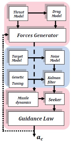
Fig.1 shows the block diagram of the target-missile model which has the following parts
The interceptor is modeled as a point in NED (North-East- Down) coordinate system with the assumption that the earth is flat. The following vector describes the missile present state
𝑀(𝑘)
= [𝑥𝑀 (𝑘) 𝑥̇ 𝑀 (𝑘) 𝑦𝑀 (𝑘) 𝑦̇ 𝑀 (𝑘) 𝑧𝑀 (𝑘) 𝑧̇𝑀 (𝑘)]𝑇 (1)
IJSER © 2015 http://www.ijser.org
International Journal of Scientific & Engineering Research, Volume 6, Issue 2, February-2015 1210
ISSN 2229-5518
1 ∆ 0
⎡0 1 0
0 0 0
0 0 0⎤
𝑥𝑇 (𝑘)
⎡𝑥̇ 𝑇 (𝑘 ⎤
⎢ ⎥ ⎢ ⎥
𝑇(𝑘 + 1) =
0 0 1
∆ 0 0
⎢𝑦𝑇 (𝑘)⎥
(4)
⎢0 0 0
⎢0 0 0
⎣0 0 0
1 0 0⎥ ⎢𝑦̇ 𝑇 (𝑘)⎥
0 1 ∆⎥ ⎢𝑧𝑇 (𝑘)⎥
0 0 1⎦ ⎣𝑧̇𝑇 (𝑘)⎦
In three second before the impact, the target begins a six g turn in the x-y plane. In this case the modified next state is
1 𝐴 0
⎡0 𝐶 0
𝐵 0 0
−𝐷 0 0⎤
𝑥𝑇 (𝑘)
⎡𝑥̇ 𝑇 (𝑘 ⎤
⎢ ⎥ ⎢ ⎥
𝑇(𝑘 + 1) =
0 𝐵 1
𝐴 0 0
⎢𝑦𝑇 (𝑘)⎥
(5)
⎢0 𝐷 0
⎢0 0 0
⎣0 0 0
𝐶 0 0⎥ ⎢𝑦̇ 𝑇 (𝑘)⎥
0 1 ∆⎥ ⎢𝑧𝑇 (𝑘)⎥
0 0 1⎦ ⎣𝑧̇𝑇 (𝑘)⎦
𝐴 = sin(𝜔𝑡 ∆), 𝐵 = {1−cos(𝜔𝑡 ∆)}, 𝐶 = cos(𝜔 ∆),
![]()
![]()
𝜔𝑡
![]()
𝐷 = sin(𝜔𝑡 ∆), 𝜔𝑡 =
𝜔𝑡
𝑡
𝑟𝑡𝑢𝑟𝑛
�𝑥̇𝑇(𝑘)2 +𝑦̇𝑇 (𝑘)2
where ωt is the target angular turn rate, aturn = 6g
Fig.1 Block diagram of target-interceptor scenario
The next state is described by
1- The thrust is 23000 Newton for the first 6 seconds. It accel- erates the missile up to 1100 m/sec.
2- The drag is composed of induced drag and parasitic drag.
The induced drag due to shape of missile and dynamic pres- sure is![]()
𝑚�𝑟2 +(𝑟𝑀𝑒 −𝘨)2
𝑀(𝑘 + 1) =
𝐹𝑟𝑛 = 𝑄 ∗ 0.25
![]()
𝑆𝑟𝑛𝑓 (6)
1 ∆ 0
0 0 0 ⎡𝑥𝑀 (𝑘)
0.5𝑥̈𝑀 (𝑘)∆2
Where m is the mass of the missile, aMa and aMe are azimuth
⎡0 1 0
0 0 0⎤
⎥
𝑥̇ 𝑀 (𝑘)⎥
⎢ 𝑥̈ 𝑀 (𝑘)∆ ⎥
and elevation command accelerations for the missile, g is the
⎢0 0 1
∆ 0 0 ⎢𝑦𝑀 (𝑘)
⎢0.5𝑦̈𝑀 (𝑘)∆2 ⎥
gravitational acceleration, S
is the cross sectional area of the
⎢ ⎥ + ⎢
⎥ (2)
ref
⎢0 0 0
1 0 0⎥ ⎢𝑦̇ 𝑀 (𝑘)
⎢ 𝑦̈ 𝑀 (𝑘)∆ ⎥
missile, Q is a dynamic pressure. The parasitic drag is
⎢0 0 0
0 1 ∆⎥ ⎢𝑧𝑀 (𝑘)⎥
⎢0.5𝑧̈𝑀 (𝑘)∆2 ⎥
⎣0 0 0
0 0 1⎦ ⎣𝑧̇𝑀 (𝑘)⎦
⎣ 𝑧̈𝑀 (𝑘)∆ ⎦
𝐹𝑟𝑝
= 𝑄 ∗ 𝐶𝑟𝑝
∗ 𝑆𝑟𝑛𝑓
(7)
Where ∆ is discrete time step size
The present state of the target is represented by
𝑇(𝑘) =
[𝑥𝑇 (𝑘) 𝑥̇ 𝑇 (𝑘) 𝑦𝑇 (𝑘) 𝑦̇ 𝑇 (𝑘) 𝑧𝑇 (𝑘) 𝑧̇𝑇 (𝑘)]𝑇 (3)
Cdp is a parasitic drag coefficient. The total drag is the sum of
induced drag and parasitic drag.
Fig. 2 shows the engagement geometry for PN law. The main concept of proportional navigation is to keep line of sight con- stant by eliminating line of sight rate. It can be expressed as
The next state is
𝑎𝑐 (𝑡) = 𝑁𝑣
𝑐𝑙
𝜆̇ (8)
IJSER © 2015 http://www.ijser.org
International Journal of Scientific & Engineering Research, Volume 6, Issue 2, February-2015 1211
ISSN 2229-5518
where at is a target acceleration, ηt is a target heading relative to line of sight, ηm is a missile look angle, N is a navigation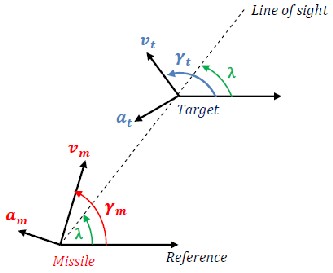
constant. In the case of Kalman filter tuning, this guidance law
can modified to be
𝑎𝑐 (𝑡) = �𝑇𝑓1 𝑎𝑡 �![]()
cos�𝑇𝑓2 𝜂𝑡�
cos 𝜂𝑚
+ 𝑁![]()
�𝑇𝑓3 𝑣𝑐𝑙��𝜆̇ 𝑇𝑓4 �
cos 𝜂𝑚
(11)
Fig.2 Engagement geometry of PN law
,where ac (t) is the acceleration command, N is the navigation ratio, vcl is the estimated closing velocity, λ̇ is the estimated
line of sight rate. In the case of Kalman filter tuning, this guid-
ance law can modified to the form
𝑎𝑐 (𝑡) = 𝑁(𝑇𝑓1 𝑣𝑐𝑙 )(𝑇𝑓2 𝜆̇ ) (9)
Where Tf1and Tf2 are the tuning factors for both estimated
closing velocity and estimated line of sight rate respectively,
and there values lies between (0.8,1.2) and genetic algorithm is
used to find the optimum values of them.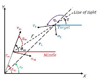
Fig.3 Engagement geometry of DG law
Fig.3 shows the engagement for DG law. It can be expressed as
The Kalman filtering algorithm is a state estimator known as the workhorse of estimation. In this paper, it is used to es- timate the position, velocity, and acceleration of noisy estima- tion of position. It can be broken into prediction and correction phases [8].
At the end of the current state k the prediction phase occurs. It computes a next state (k+1) parameters and covariance using the current (k ) state estimate. The measurements are taken between the prediction and correction phases, and then the correction phase calculates a corrected state estimate and co- variance for time (k +1).
Noisy line of sight angle and range are generated with
𝜃𝐿𝑛𝑛 = 𝜃𝐿 + 𝜎𝜃𝐿 𝑛𝑟𝑟𝑛𝑟 (12)
𝑟𝑛𝑛 = 𝑟 + 𝜎𝑟 𝑛𝑟𝑟𝑛𝑟 (13)
𝑛𝑟𝑟𝑛𝑟 is a random value, drawn from a zero mean Gaussian
distribution with variance of one. The standard deviations are
𝜎𝜃𝐿 = 𝑓𝑛𝑛𝑛𝑛𝑛 𝜎𝜃𝐿_𝑏𝑟𝑛𝑛 (14)
𝜎𝑟 = 𝑓𝑛𝑛𝑛𝑛𝑛 𝜎𝑟_𝑏𝑟𝑛𝑛 (15)
𝑓𝑛𝑛𝑛𝑛𝑛 is a factor used to determine the gain of noise. The
baseline range and line of sight angle standard deviations are
defined as 10 meters and 1 m.rad respectively, [9].
The guidance system of the missile responds to noise with slight guidance accelerations commands which produce an induced drag. Thus the total drag increases exponentially with increasing of missile velocity which leads to produce dramatic performance deterioration.
The state prediction equation is
𝑥�(𝑘 + 1|𝑘) = 𝐹(𝑘)𝑥�(𝑘|𝑘) + 𝐺(𝑘)𝑢(𝑘) (16)
𝑎𝑐 (𝑡) = ‖𝑎𝑡 ‖![]()
cos 𝜂𝑡
cos 𝜂𝑚
+ 𝑁![]()
𝑣𝑐𝑙𝜆̇
cos 𝜂𝑚
(10)
𝐹(𝑘) is the state transition matrix, u(k) is a deterministic input vector, and G(k) is an identity matrix used to weight input.
IJSER © 2015 http://www.ijser.org
International Journal of Scientific & Engineering Research, Volume 6, Issue 2, February-2015 1212
ISSN 2229-5518
The predicted state estimate covariance estimates the accuracy of the predicted state estimate based on the corrected state covariance and process covariance of the previous time step k. It is given by
𝑃(𝑘 + 1|𝑘) = 𝐹(𝑘)𝑃(𝑘|𝑘)𝐹(𝑘)ʹ + 𝑄(𝑘). (17)
Q(k) is a process covariance. The predicted measurement es-
timate is defined as the filter expectation of the state (k+1)
measurement based on the predicted state estimate, It is given by
𝑧̂(𝑘 + 1|𝑘) = 𝐻(𝑘 + 1)𝑥�(𝑘 + 1|𝑘) (18)
𝐻(𝑘 + 1) is the measurement extraction matrix which repre-
sents the measurement from the state vector for time (k+1).
In this phase the corrected state estimate and covariance are generated by updating the predicted state estimate and covar- iance. This phase contains calculation of residual of the meas- urements which is defined as the difference between the real measurements and the predicted measurements
𝑟(𝑘 + 1) = 𝑧(𝑘 + 1) − 𝑧̂(𝑘 + 1|𝑘) (19)
The measurement z(k + 1)represents state translation and
transients during the time elapsed between steps as well as
measurement noise. It can be represented as
𝑧(𝑘 + 1) = 𝐻(𝑘 + 1)𝑥(𝑘 + 1) + 𝑤(𝑘 + 1) (20)
𝑤(𝑘 + 1) is the filter gain. It determines the influence of pre-
vious estimates and the current measurement on the predicted
state estimate and covariance.
𝑊(𝑘 + 1) = 𝑃(𝑘 + 1|𝑘)𝐻(𝑘 + 1)′ 𝑆(𝑘 + 1)−1 (21)
The covariance of the measurement residual is
𝑆(𝑘 + 1) =
𝑅(𝑘 + 1) + 𝐻(𝑘 + 1)𝑃(𝑘 + 1|𝑘)𝐻(𝑘 + 1)′ (22)
The next step is correction of state estimation. It modifies the
predicted state by a magnitude according to the measurement
residual and the filter gain, it is
𝑥�(𝑘 + 1|𝑘 + 1) = 𝑥�(𝑘 + 1|𝑘) + 𝑊(𝑘 + 1)𝑟(𝑘 + 1) (23)
Finally, the corrected state estimation covariance is
𝑃(𝑘 + 1|𝑘 + 1) =
𝑃(𝑘 + 1|𝑘) − 𝑊(𝑘 + 1)𝑆(𝑘 + 1)𝑊 ′(𝑘 + 1) (24)
for the half of range and new constant values for the rest of the range until interception point. So the optimization problem in this case is to find the optimum values for four variables which achieve the desired cost function.
Second, in the case of differential geometry (DG) guidance
law, the scale of the optimization problem is two time the pre-
ceding one. Since the estimated values to be tuned are target
acceleration, target lead angle, closing velocity, and line of
sight rate. Every estimated value has its tuning factor that is divided into two values as explained in PN law. Thus the op- timization problem in DG law is to find the optimum values for eight variables that achieve the desired cost function.
The objective function is to decrease the miss distance at long ranges to achieve miss distance less than kill radius (5m)
which also decrease the miss distance at less ranges at the same target direction and leads to reduce the minimum effec- tive range below the minimum value. An optimization process is formulating using binary genetic algorithm Matlab program in reference [10].
The main object of Kalman filter is estimating the target range and line of sight. The estimation errors are increased in the presence of noise and causes performance degradation like decreasing the maximum effective range, increasing minimum effective range and increasing the miss distance.
Fig.5 shows the effect of noise of the maximum effective range with different values of noise factors. The values of maximum effective range are taken every thirty degrees and beginning with zero up to 180 degree and drawing a mirror figure from
180 to 360 degree. The figure shows performance degradation
in the direction of 30 degree and 60 degrees due to estimation errors.
To enhance the performance of PN law, the estimates values for both ranges and line of sight are multiplied by correction factors to eliminate estimation errors. The correction factor of range is divided into two values for the first half and the se- cond half of range. The correction factor of line of sight is di- vided with the same way. The values of the correction factor lie between 0.8 and 1.2. The genetic algorithm is used to find the optimum values of the correction factors.
Fig.4 shows the flow chart of the optimization process.
First, in the case of proportional navigation there are two fac-
tors to tune the estimated values of line of sight rate and clos-
ing velocity. The tuning factors have specific constant values
IJSER © 2015 http://www.ijser.org
International Journal of Scientific & Engineering Research, Volume 6, Issue 2, February-2015 1213
ISSN 2229-5518
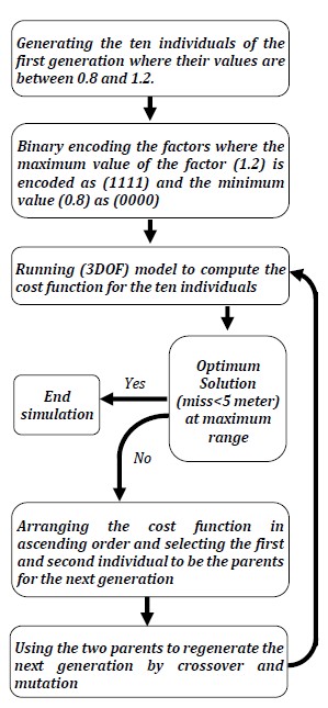
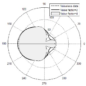
Fig.5 PN performance at different values of noise factor
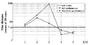
Fig.6 KF performance for at low ranges (NF=2)
Fig.7 has the same comparison as Fig.6 but at long ranges. The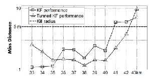
figure shows that tuning Kalman filter performance increases the maximum effective range from 40 Km to 41 Km and re- duces the miss distance at a lot of ranges.
Fig.4 Flow chart of optimization process
Fig.6 shows the performance of Kalman filter and tuned Kal- man filter in the direction of 30 degree and noise factor=2 for low ranges. The figure shows that no change in the minimum effective range which is equal to five kilometers but the aver- age values of miss distances which resulting from run the simulation 20 times are decreased at the ranges (1, 2, and 3 kilometers).
Fig.7 KF performance at long ranges (NF=2)
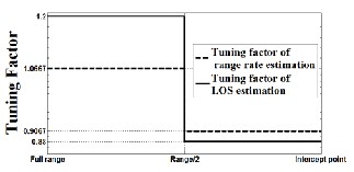
Fig.8 contains the values of multiplied factors for both LOS
estimated and range estimated and their distribution along the range between target and interceptor
IJSER © 2015 http://www.ijser.org
International Journal of Scientific & Engineering Research, Volume 6, Issue 2, February-2015 1214
ISSN 2229-5518
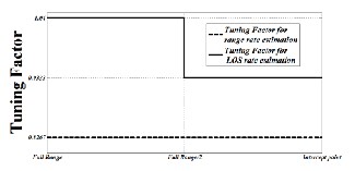
Fig.8 Tuning factors distribution along the range (NF=2)
The noise affects the performance of Kalman filter, so increas- ing noise factor causes performance degradation of Kalman filter and it needs to be tuned again to adapt increasing the noise gain. Therefore the same steps are taken again using genetic algorithm to find the optimum values of tuning factor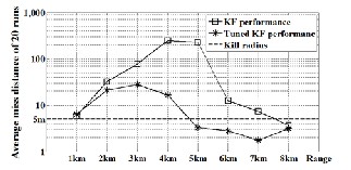
Fig.9 KF performance at low ranges (NF=4)
Fig.9 indicates the values of the average miss distances of 20 runs at low ranges. The figure shows that tuning Kalman filter reduce the minimum effective range from 8 to 5 Km and also minimizes the miss distances at all ranges for noise factor=4. Fig.10 KF performance at long ranges (NF=4)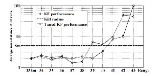
Fig.10 KF performance at long ranges (NF=4)
Fig.11 Tuning factor distribution along the range (NF=4)
Fig.10 shows the same data but for long ranges which also
indicates enhancement of maximum effective range from 38 to
40 Km. Fig.11 shows the tuning factors that achieve the opti- mum performance for both low and long ranges.
Fig.12 shows 3D representation of genetic algorithm search results of range 40 Km, heading 30 degree, and noise factor=4. The optimum (minimum) average miss distance is the first individual of the seventeenth generation
Fig.12- 3D plot of genetic algorithm search results
Fig.13 shows the influence of increasing noise factor on the performance of Kalman filter with differential geometry law. The figure shows that differential geometry law is very sensi- tive to increasing the gain of noise which causes a slight reduc- tion in the effective area in the case of noise factor equal one, and great shrink in area at noise factor equal two.
As mentioned before, tuning of Kalman filter by correction factors enhances the performance. In the case of differential geometry law there are four estimated values need to be tuned. The first value is the target acceleration and the rest values are target lead angle, closing velocity, and line of sight rate respectively.
IJSER © 2015 http://www.ijser.org
International Journal of Scientific & Engineering Research, Volume 6, Issue 2, February-2015 1215
ISSN 2229-5518
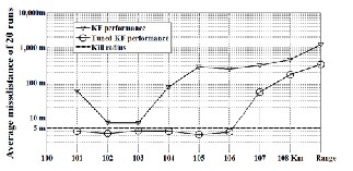
 Fig.16 KF performance for long ranges (NF=2)
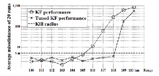
Fig.13 The effect of noise on effective areas 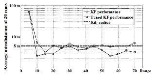
Fig.17 KF performance for low and medium ranges (NF=2)
Fig.16 and Fig.17 show the performance of Kalman filter and tuned Kalman filter when the noise factor =2 for long, medi- um, and low ranges. The target heading is 180 degree. The two figures show enhancement in performance due to using tuned Kalman filter.
Fig.14 KF performance at long ranges (NF=1)
Fig.14 shows the results for both tuned and unturned values for Kalman filter for noise factor one and target heading 180 degrees. The results indicate increasing in the maximum effec- tive range from 105 to 108 Km.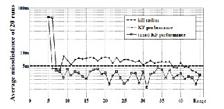
Fig.15 KF performance for low and medium ranges (NF=1)
Fig.15 shows the same results for low ranges which indicate improvement of minimum effective range from 41 Km to 7
Km by decreasing the miss distance smaller than 5 meters (the
kill radius).
TABLE I
DISTRIBUTION OF THE TUNING FACTORS ALONG THE RANGE
Noise Factor=1 | Noise Factor=2 | |||
First half | Second half | First half | Second half | |
Target ac- celeration | 1.2 | 0.929 | 0.8516 | 0.84 |
Target lead angle | 1.1 | 0.9806 | 1.084 | 1.2 |
Closing ve- locity | 0.85 | 0.8 | 1.09 | 1.18 |
LOS rate | 1.1355 | 0.81 | 1.161 | 0.968 |
In Table.1, the tuning factors for estimated values of target acceleration, target lead angle, closing velocity, and line of sight rate are shown for both noise factor one and two respec- tively and target heading=180˚.
IJSER © 2015 http://www.ijser.org
International Journal of Scientific & Engineering Research, Volume 6, Issue 2, February-2015 1216
ISSN 2229-5518
Fig.18.3D plot of genetic algorithm search results
Fig.18 shows 3D representation of genetic algorithm search results of target heading 180 degree, and noise factor=2. The optimum (minimum) average miss distance is the first indi- vidual of the sixteenth generation.
1-The performance of Kalman filter with proportional naviga- tion law is enhanced by tuning factor which is found using genetic algorithm.
2- A genetic algorithm is used also to find the optimum tuning factor for differential geometry guidance law which reduces miss distance, increases the maximum effective range, and decreases the minimum effective range.
3- A differential geometry guidance law is very sensitive to increase the noise gain (noise factor) more than proportional navigation, thus tuning factors plays an important rule to en- hance the performance especially with differential geometry law.
1- A noise causes undesirable effects on the performance of the guidance law.
2- A Kalman filter is used to get estimated values of the guid- ance law and reduces the bad effects of the noise.
3- The performance of Kalman filter is changed by multiply the estimated value by tuned factor lie between 0.8-1.2
4-A genetic algorithm is used to find the optimum values of
tuned factors in every direction of target heading.
5- For future works, the tuning factors in all directions can be calculated and used as training data to train the neural net- works such that these factors can be used online.
[1] C.K. Chui , G. Chen. ” Kalman Filtering with Real-Time Applications”.
Fourth Edition, 2009
[2] C. Wren, A. Azarbayejani, T. Darrell, and A. Pentland. Pfinder. “ Real- time tracking of the human body”. IEEE Transactions on PAMI, 19(7):780–
785, 1997.
[3] H. Ekenel and A. Pnevmatikakis. “Video-Based Face Recognition Evalua- tion “ CHIL Project. International Conference of Pattern Recognition, 2006.
[4] D. Beymer, P. McLauchlan, B. Coifman, and J. Malik. “A real-time comput- er vision system for measuring traffic parameters”. In Proc. CVPR, pages
495–501, 1997.
[5] G.D. Sullivan. “Model-based vision for traffic scene using the ground-plane constraint”. Real-time Computer Vision,1994. D. Terzopoulos and C. Brown (Eds.).CUP
[6] D R Magee.”Tracking Multiple Vehicles using Foreground, Background and Motion Models”. December 2001 European Conference on Computer
Vision, May 2002.
[7] Nilanjan Patra, Kaushik Halder, Avijit Routh, Abhro Mukherjee, Satyabrata Das, “Kalman Filter based Optimal Control Approach for Attitude Control of a Missile” International Conference on Computer Communication and Informatics, 2013.
[8] Osborn, Adam M.” A study into the effects of Kalman filtered noise in advanced guidance laws of missile Navigation”, Thesis, Naval Postgradu-
ate School, 2014.
[9] Daniel Perh. ”A study into advanced guidance laws using computational methods” Thesis, Naval Postgraduate School, 2011.
[10] L. Haupt Randy, Sue Ellen Haupt, “ Practical Genetic Algorithms “(A John
Wiley & Sons, INC.Publication, second edition, 2004)
IJSER © 2015 http://www.ijser.org