is 0.59 given by Betz limit. In practice because of tip loss, wake swirl loss and profile drag loss the value of Cp being lowered than this limiting value. (2)
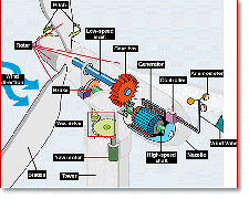
Figure 1: Wind Turbine Diagram
International Journal of Scientific & Engineering Research, Volume 5, Issue 3, March-2014
ISSN 2229-5518
1010
Efficient Wind Turbine Blade Design
Adnan Miski
Abstract— There are several issues with designing an energy saving wind turbine; the first one is to find the optimal blade length to achieve the demanded power (60 W). In order to do that, we need to calculate the unknown variables which is the monthly mean velocity (Vm), typical value for coefficient of performance and efficiency (Cp,) and the Swept Area of Blades (A). The second problem is to find the typical air density and the capacity factor to achieve optimal power which is 60 Watts. Third problem is finding the tip speed ratio and the required number of blades for the turbine we are going to design. Fourth problem is the determination of blade Cord width "C(r)" and the blade twist angle "". The last issue is to find the Wind turbine power curve. The paper proposed an efficient wind turbine design taking into consideration all the above mentioned issues.
Index Terms— Electric Generator, Efficient Blade Design, Energy Saving, optimal power, Tip Speed Ration, Weibull Distribution, Wind
Turbine Design.
—————————— ——————————
here are several issues with designing an energy saving wind turbine; the first one is to find the optimal blade length to achieve the demanded power (60 W). In order to
do that, we need to calculate the unknown variables which is the monthly mean velocity (Vm), typical value for coefficient of performance and efficiency (Cp,) and the Swept Area of Blades (A). The second problem is to find the typical air densi- ty and the capacity factor to achieve optimal power which is
60 Watts.
Third problem is finding the tip speed ratio and the required number of blades for the turbine we are going to design. Fourth problem is the determination of blade Cord width "C(r)" and the blade twist angle "". The last issue is to find the Wind turbine power curve.
Detailed Wind turbines, like aircraft propeller blades, turn in the moving air and power an electric generator that supplies an electric current. Simply stated, a wind turbine is the oppo- site of a fan. Instead of using electricity to make wind, like a fan, wind turbines use wind to make electricity. The wind turns the blades, which spin a shaft, which connects to a gen- erator and makes electricity. (1)
For Horizontal turbine components include (Figure 1):
Blade or rotor, which converts the energy in the wind
to rotational shaft energy;
A drive train, usually including a gearbox and a gen-
erator;
A tower that supports the rotor and drive train; and
Other equipment, including controls, electrical cables,
ground support equipment, and interconnection equipment. (1)
Cp is called the power coefficient. Cp is the percentage of power in the wind that is converted into mechanical energy. The maximum achievable coefficient of performance Cp max
is 0.59 given by Betz limit. In practice because of tip loss, wake swirl loss and profile drag loss the value of Cp being lowered than this limiting value. (2)
Figure 1: Wind Turbine Diagram
Energy conversion efficiency is the ratio between the useful output of an energy conversion machine and the input, in en- ergy terms.
![]() (1)
(1)
The actual amount of energy that can be extracted from the wind is less than the theoretical amount of energy available with the theoretical limit being about 60%. A typical efficiency for a wind turbine is about 40% which is about 40% of the power available in the area swept by the wind turbine blades.(2)
The density of dry air at sea level is 1.225 kg/m3 or about
1/800th the density of water. But as altitude increases, the density drops dramatically. This is because the density of air is proportional to the pressure and inversely proportional to temperature. And the higher you go into the atmosphere, the lower the pressure gets. Pressure is approximately halved for each additional increase of 56 km in altitude. (3)
IJSER © 2014
International Journal of Scientific & Engineering Research Volume 5, Issue 3, March-2014
ISSN 2229-5518
1011
The power output from a wind turbine given by:
Table 3: Calculation for the monthly power![]()
(2)
Where,
The number of blades "B" is inversely proportional to the square of the tip speed ratio “λ” for a given blade radius and of the blade outer portion "C" is given by:![]()
(3)
Where,
The mean velocity at hub height 10m will be calculated. A 20m height will also be calculated as shown in table 1.
Table 1: Calculating the mean velocity at 10m & 20m
The shape of The Weibull identified with the function (K) and the Scale of The Weibull function (C) as parameters and the wind velocity (v). A table constructed to show the variation of f (v) and Pwind (v) (watt/m2) with the velocity by using these values for C and K, 4.1 and 2.14 respectively.
Table 4: Constructed variation of f (v) and Pwind (v)
Month | K | C | Mean Velocity at 10m | Mean Velocity at 20m |
January | 2.1 | 4.17 | 3.7 | 4.1 |
February | 2.05 | 4.27 | 3.8 | 4.2 |
March | 2.25 | 4.46 | 4.0 | 4.4 |
April | 2.25 | 3.35 | 3.0 | 3.3 |
May | 2.37 | 4.2 | 3.7 | 4.1 |
June | 2.45 | 4.34 | 3.8 | 4.2 |
July | 2.4 | 4.02 | 3.6 | 3.9 |
August | 2.55 | 3.97 | 3.5 | 3.9 |
September | 2.4 | 3.82 | 3.4 | 3.7 |
October | 2.05 | 3.16 | 2.8 | 3.1 |
November | 2.1 | 3.43 | 3.0 | 3.4 |
December | 2 | 3.9 | 3.5 | 3.8 |
Table 2: Design variables
Z (m) | 10 |
Zr (m) | 20 |
Air Density (kg/m3) | 1.225 |
Coefficient of Performance | 0.35 |
Efficiency | 0.65 |
Calculating the monthly delivered power for different blade lengths (R1= 0.5, R2=1, R3=1.5, R4 = 2 and R5=2.5) at hub height 20m by using equation 1 as shown in table 3.
Then we draw the probable generated wind power density Pe(v) as a function of the wind velocity as shown in figure 3 by using these values for C and K , 4.1 and 2.14 respectively.
IJSER © 2014
International Journal of Scientific & Engineering Research Volume 5, Issue 3, March-2014
ISSN 2229-5518
1012
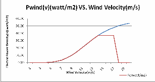
Figure 2: The Relation between the Power and the Velocity
Last but not least the calculation of the percentage capacity factor "CF" and the estimation of the effect of changing the weibull parameter "c" by 10 % on the calculated capacity factor as shown In table 6.
Table 5: The result of Vmp,Vr and CF and effect of 10% change
f(Vmp) | f(VR) | P(Vmp,k,c) | P(VR,k,c) | CF |
0.22 | 0.06 | 1.92 | 5.22 | 0.37 |
CF (+10%) | ||||
0.20 | 0.06 | 2.32 | 6.32 | 0.37 |
CF (-10%) | ||||
0.24 | 0.07 | 1.55 | 4.23 | 0.37 |

Using the swept area from stage 1 (19.652 m2) the upper and lower bound for the number of blades sketched as shown be- low:
Figure 3: Lower bound for # of blades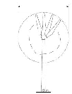
Figure 4: Upper bound for # of blades
The lower number of blades is 1 while the upper number of blades is equal 8 for the swept area of 19.652 m2.
Table 6: coefficient of performance Cp for different tip speed
1 Blade | 2 Blades | 3 Blades | 4 Blades | |
Linda | Cp/Cmax | Cp/Cmax | Cp/Cmax | Cp/Cmax |
4 | 0.44 | 0.49 | 0.51 | 0.52 |
4.5 | 0.41 | 0.46 | 0.47 | 0.48 |
5 | 0.38 | 0.42 | 0.43 | 0.44 |
5.5 | 0.35 | 0.38 | 0.39 | 0.40 |
6 | 0.32 | 0.34 | 0.35 | 0.35 |
6.5 | 0.28 | 0.30 | 0.31 | 0.31 |
7 | 0.24 | 0.26 | 0.26 | 0.26 |
7.5 | 0.20 | 0.21 | 0.22 | 0.22 |
8 | 0.16 | 0.17 | 0.17 | 0.17 |
8.5 | 0.12 | 0.12 | 0.12 | 0.12 |
9 | 0.07 | 0.08 | 0.08 | 0.08 |
The relation between the blades number and the coefficient of performance Cp for different tip speed ratios is shown in fig- ure 5.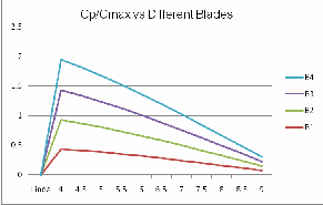
Figure 5: relation between the blades number and the coefcient of performance Cp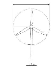
The number of blades we chose is 3 as sketched in figure 6. The reason for choosing 3 because compared to the single and two-bladed turbines, the three-blade rotor has a much smoother power output, more efficient, higher energy yield and a balanced gyroscopic force and a much better mechanical system. The tip speed ratio we chose is 5 because it’s within the range of tip ratios which is 5-8 also we chose 5 because it has the maximum Cp/Cmax with the minimum number of blades possible which is 3 blades.
The coefficient of performance Cp as a function of the number of blades "B" for different tip speeds.
IJSER © 2014
http://www.ijser.org
Figure 6: Three blades turbine
International Journal of Scientific & Engineering Research Volume 5, Issue 3, March-2014
ISSN 2229-5518
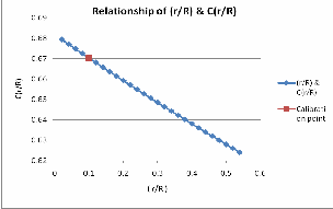
A model was constructed to predict the decrease of the cord width as a cooling of a cold drink. The calibration points used were, R=2, (r/R) 0.1 and C(r/R) 0.67. Goal seek function was used to create the model in the excel sheet and the results is shown in table 9 also a graph is drawn (figure 7) for better representation of the data.
Table 7: Values used in the model
Figure 7: Relationship between (r/R) & C(r/R)
1013
Table 8: The decrease of the cord width C(r/R)
The cord width as a function of (r/R) after 10 steps for (r/R) is shown in table 10. The beta as a function of (r/R) after 10 steps for (r/R) is shown at the same table with the thickness of the blade.
Table 9: Values for cord width, and thickness of the blade
(r/R) | C (r/R ) | ( r/R ) | t (r/R) |
0.1 | 0.16 | 48.10 | 0.047 |
0.2 | 0.16 | 28.66 | 0.027 |
0.3 | 0.52 | 18.93 | 0.073 |
0.4 | 0.42 | 13.40 | 0.054 |
0.5 | 0.35 | 9.90 | 0.042 |
0.6 | 0.30 | 7.50 | 0.035 |
0.7 | 0.26 | 5.75 | 0.029 |
0.8 | 0.23 | 4.43 | 0.026 |
0.9 | 0.20 | 3.40 | 0.023 |
1 | 0.18 | 2.56 | 0.020 |
The value of Cl is 1.00 after using the calibration points, R=2, (r/R) 0.1 and C(r/R) 0.67 the value was obtained by the goal seek function in Excel. The value of is 5.03 after using the calibration points, R=2, (r/R) 0.1 and (r/R) 48.1 the value is also obtained by the goal seek function. The data in the Ex- cel is shown in the table below:
Table 10: Values of Cl and after using goal seek
| 5 |
B | 3 |
Cl | 0.30 |
| 5.03 |
dx | 0.02 |
The cumulative probability distribution function is drawn by using San Jose weibull parameters as shown in the figure be- low:
IJSER © 2014
International Journal of Scientific & Engineering Research Volume 5, Issue 3, March-2014
ISSN 2229-5518
1014
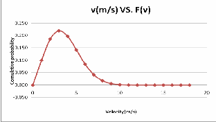
Figure 8: The cumulative probability distribution function
A stochastic model is built in the excel sheet to generate a ran- dom PN(v), then the corresponding random wind velocity is calculated as shown in table 13. The V (H) value in table 12 is calculated and the risk which is counter over iterations equals
0.134328.
Table 11: A stochastic model to generate a random PN(v)
Count | 63 |
Reset | 1 |
Iterations | 469 |
Random Number | 0.236791 |
Random Velocity | 2.22451 |
Vc(H) | 1.5 |
V(H) | 1.656134 |
P(v) | 1.391114 |
P(vc) | 1.033594 |
Risk | 0.134328 |
The power corresponding to the random wind velocity is shown in the table below:
Table 12: Random wind velocity
The velocity equal to the cut in velocity "P(Vc)" is calculated in table 12. The stochastic model is used to predict the frequency of obtaining a power lower than "P(Vc)" also shown at table
12. The percentage wind power loss due to the cut in speed is
35%. The power curve is drawn as shown below: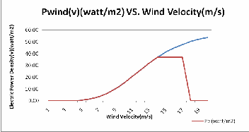
Figure 9: Power curve
The highest power rate achieved at R5 in February where P =
168.7 W. The 2.5 radius is the best for our design because most of the time it will give us what we want as shown in figure 10.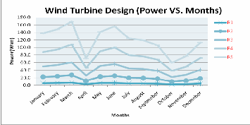
Figure 10: Monthly delivered power for different blade lengths
After calculations we came to found that the appropriate radi- us is 2.5 meters. As you noticed that some points of the curve are equals 60 watts, but most of the points are above 60 watts, and because the power will be saved when it’s more than 60 watts, we chose the 2.5 meters radius curve.
Changing the parameter “c” does not affect the capacity factor it remains at 37% as shown in table 6. Therefore, the value of Vmp, Vmax, Vm, VR, VC and VF also does not change.
The tip speed ratio we chose is 5 because it has the maximum Cp/Cmax with the minimum number of blades possible, and the number of blades we choose is 3 because compared to the single and two-bladed turbines, the three-blade rotor has a
IJSER © 2014
International Journal of Scientific & Engineering Research Volume 5, Issue 3, March-2014
ISSN 2229-5518
1015
much smoother power output, more efficient, higher energy yield and a balanced gyroscopic force and a much better me- chanical system.
The value of Cl is 1.00 after using the calibration points, R=2, (r/R) 0.1 and C(r/R) 0.67. The value of is 5.03 after using the using the calibration points, R=2, (r/R) 0.1 and (r/R)
48.1.
The velocity equal to the cut in velocity "P(Vc)" is calculated is equal to 1.033594 and the risk is 0.132911. The stochastic mod- el is used to predict the frequency of obtaining a power lower than "P(Vc)" as shown at table 12. The percentage wind power loss due to the cut in speed is 35%.
After carful calculations we came to find that the best length for the blade is 2.5m because it provides the required power rate for most of the time and it’s the best option to save ener- gy. Capacity factor remains at 37% after ±10% changes on “c” parameter.
Tip speed ratio will be 5 and the number of blades going to be
3 because three blades has a much smoother power output, more efficient, higher energy yield and a balanced gyroscopic force compared to the single and two-bladed turbines. The value of left coefficient is 1.00 and the value of angle of attack is 5.03. The percentage wind power loss due to the cut in speed is 35%.
[1] http://windeis.anl.gov/guide/basics/index.cfm (visited at 8:21P.M on Nov,2 2013)
[2] http://guidedtour.windpower.org/en/core.htm (visited
at 10:02P.M on Nov,10 2013)
[3] http://www.windenergyturbine.net/cms1/prva.go?stid=
6&idpodstran=8 (visited at 1:30P.M on Nov,13 2009)
[4] http://hypertextbook.com/facts/2000/RachelChu.shtml
(visited at 1:30P.M on Nov,21 2013)
IJSER © 2014