International Journal of Scientific & Engineering Research, Volume 4, Issue 12, December-2013 70
ISSN 2229-5518
An Efficient Paroxysmal Atrial Fibrillation
Prediction Method Using CWT and SVM
Ashraf Anwar1 and Hedi Khammari2
ABSTRACT—Paroxysmal Atrial Fibrillation (PAF) is the most commonly occurring arrhythmia and its prevalence increases with age. This paper presents an efficient method for detection and prediction of (PAF) using PAF prediction challenge database (afpdb) to locate normal person from person who suffers from PAF. We extract 11 features from 100 ECG recorded signals database with the aid of continuous wavelet transform (CWT), to allow accurate extraction of feature from non- stationary signal like ECG, and a Support Vector Machines (SVM) to classify the patterns inherent in the features extracted. We divide the 30-min preceding the PAF into 6 periods with 5-min each. In each suggested period we get the classification result using (SVM). The measured sensitivity, specificity, positive predictivity and accuracy show better and significant results comparable to the other results obtained in the same field in the literature.
Index Terms—PAF prediction, ECG signal, continuous wavelet transform, support vector machine, statistical parameters.
1. INRODUCTION
Paroxysmal atrial fibrillation (PAF) of the heart muscle is defined as short duration episodes of AF lasting from 2min. to less than 7 days, while chronic AF is defined as lasting more than 7 days. The main reason for this is not the immediate effect of the onset of atrial fibrillation over the patient’s health (AF detection) but the long-term effects: increase in
models are able to detect the transition to PAF events with accuracies of 70–90%, by means of records of at least tens of minutes and rather complex analysis procedures.
In the present work, several features are extracted
with the aid of CWT which convert the time domain
signal to time-frequency domain where several
IJSER
heart muscle fatigue, increase in thromboembolic
and stroke events due to the formation of blood clots
and an irregular onset that makes it hard to detect on
normal ECG tests. Thus it is necessary for
cardiologists to benefit from a robust and precise tool
that could predict the onset of such events, in order
to prevent them by defibrillation, drug treatment and anti-tachycardia pacing techniques. The automated method to predict the onset PAF is interesting topic to help treating this problem.
During recent years several researchers proposed
many techniques to predict the onset of PAF. Useful reviews describing different techniques for PAF or chronic AF prediction, from technical to clinical points of view [1-5]. The “Computers in Cardiology Challenge 2001” revealed a maximum obtained accuracy of about 80% [6-8]. Thong [9] reports a sensitivity and specificity of 89% and 91% respectively, by analysis of atrial premature complexes (that trigger 93% of PAF episodes).
Support vector machine (SVM) in recent years
has proved to be an advanced tool in solving classification [11-13], wavelets proved usefulness in feature extraction from non-stationary signal like ECG [14-17]. In general, these above prediction
————————————————
1,2Department of Computer Engineering, Faculty of Computers and
Information Technology,
Taif University, Saudia Arabia
Email: ashraaf@tu.edu.sa
features can be carefully extracted, the extracted
features are then applied to SVM to classify the
normal object from that one who suffers from PAF.
2. MATERIAL AND METHODS
The database used for this task was PAF Prediction Challenge Database 2001 from physionet.org. It consists of 3 record sets: the first one has records that begin with the letter 'n' and comes from 50 subjects who do not have documented PAF. The length of these records is 30 min. The second record that begin with letter 'p' comes from 25 subjects who have documented PAF, and it is divided into two types, the even one has a record of 30 min preceding the PAF, and the odd one has a record of 30 min. but distant from PAF. All the previous record has a continuation 5 min record with a letter 'c'. The third record contains 100 annotated recordings for testing with a letter't' of 30 min. and unknown documentation. Each record contains two channels simultaneous recorded Holter ECG signal digitized at 128 Hz with 12 bit resolution over a 20 mV range.
We used in this task both channels of the ECG
signal (100 records) to create the database
summarized in Table 1.
The block diagram of the proposed method is shown
in Fig. 1; each block is described in more details.
Table 1 The database used for PAF prediction
IJSER © 2013 http://www.ijser.org
International Journal of Scientific & Engineering Research, Volume 4, Issue 12, December-2013 71
ISSN 2229-5518
Learning set | Testing set |
Non-PAF recording(n) | PAF-recording(p-even) | PAF and Non-PAF |
30(random selected) | 30(randomly selected) | 40 (randomly selected) |
60 | 40 |
Preprocessing | | Feature | | CWT | RR and | QRS | Feature |
| | extraction-1 | | | detection | | extraction-2 |
2.1Preprocessing.
Classification using SVM
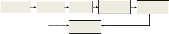
Fig. 1 Block diagram of the proposed method
The ECG signal within the database can be affected by many interfering signals such as the 50
Hz power line interference and the baseline wandering. These interfering noises are eliminated
The continuous wavelet transformation (CWT) of a signal x(t) is the convolution product of x (t) with a scaled and translated kernel function [15]
∅ = 1 ∞
t−τ

first by means of a 5-15 Hz bandpass filter. For
lowering interference noise, a median filter was
CWTx
�|s|

∫−∞ x(t)∅( s
)dt (1)
used.
2.2Continuous Wavelet Transform (CWT)
CWT allows a time domain signal to be
Where Φ((t-τ)/s)is a scaled and translated
(shifted) version of a mother wavelet which is the basic unit of wavelet decomposition, s is a scale
parameter and τ is a space parameter.
IJSER
transformed into time-frequency domain where frequency characteristics and the location of particular features in a time series may be highlighted simultaneously. Thus it allows accurate extraction of feature from non-stationary signal like ECG [14]. The CWT wavelet transform is a tool that divides up data, functions, or operators into different frequency components and then studies each component with a resolution matched to its scale. Unlike the short time Fourier transformation (STFT) the wavelet transformation has very good time and frequency resolution making it ideal in the analysis of non-stationary signals such as an ECG signal.
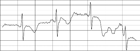
To analyze the CWT coefficients obtained for
ECG signal of PAF record and non-PAF,
predominant frequency vs. time plot of selected ECG
signal has been obtained. From these plots translation, scale and coefficient values of the peaks, which represent P, Q, R, S,T and U wave has been extracted for PAF and non-PAF records. Fig. 2 and Fig. 4 show the normal ECG signal plot and the ECG signal preceding PAF plot respectively. Fig. 3 and Fig. 5 illustrates the difference in the amplitude and duration of RR and QRS among PAF and non-PAF records at different scales with the aid of CWT.
signal n01 plot time series
R
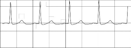
100
50 P
T
0 U
Q S
-50
-100
-150
3450 3500 3550 3600 3650 3700 3750 3800 3850
samples
Fig. 2 Normal ECG signal from n01 record
IJSER © 2013 http://www.ijser.org
International Journal of Scientific & Engineering Research, Volume 4, Issue 12, December-2013 72
ISSN 2229-5518
200
0
CWT of n01 plot scale5

-200
0 50 100 150 200 250 300 350 400
CWT of n01 plot scale 10

200
0
-200
0 50 100 150 200 250 300 350 400
CWT of n01 plot scale 50

200
0
-200
0 50 100 150 200 250 300 350 400
Fig. 3 CWT of the normal record at scales 5, 10, 50
300
200
100
signal p08 plot time series
0
-100
-200
-300
-400
-500
-600
-700
IJSER
3450 3500 3550 3600 3650 3700 3750 3800 3850
samples
Fig. 4 ECG signal preceding PAF (record p08)
400
200
0
-200
-400
400
200
0
-200
-400
CWT of p08 plot scale 5

50 100 150 200 250 300 350

CWT of p08 plot scale 10
0 50 100 150 200 250 300 350 400
CWT of p08 plot scale 50

400
200
0
-200
-400
0 50 100 150 200 250 300 350 400
2.3Feature Extraction.
Fig. 5 CWT of the PAF record at scales 5, 10, 50
(3) Sigdiff: difference between the maximum signal
We utilized 11 features: 3 (1- 3) related to signal statistical and 8 (4-11) by mean of continuous wavelet transform as follows:
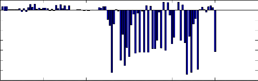
(1) Sigmean: mean value of the signal during all period (30 min), the histogram of the obtained results
is illustrated in Fig. 6. We can note that most of PAF
records have a high negative value.
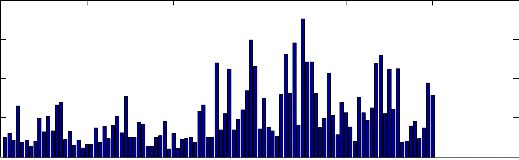
(2) Sigstd: the standard deviation of the recorded
signal, the histogram of the obtained results is
illustrated in Fig. 7. We can note that most of PAF
records have a high positive value.
and the minimum signal, the histogram of the obtained results is illustrated in Fig. 8. We can note that most of PAF records have a small positive value. (4) RRno: number of RR interval inside each period. We first detect R peak inside each period, and with the aid of CWT, we can discriminate the extremes values and their locations.
(5) RRdiff: The difference between max. RR interval
and min. RR interval inside each period.
(6) RRmax : maximum values of RR interval inside each period
IJSER © 2013 http://www.ijser.org
International Journal of Scientific & Engineering Research, Volume 4, Issue 12, December-2013 73
ISSN 2229-5518
(9) RRmean: mean values of RR interval inside each period
(7) RRrms : root mean square values of RR
interval inside each period
(8) Ramp : mean value of R peak inside each
period
(10) RRstd : standard deviation of RR interval inside each period
(11) QRSmean: mean value of QRS duration inside each period
10
0
-10
-20
-30
-40
-50
-60
mean strength of the signal, 30 min before PAF
-70
0 20 40 60 80 100 120
records(1-50 normal, 50-100 PAF)
Fig. 6 Histogram of the mean signal for all records.
std of the signal, 30 min before PAF
200
150
100
0
IJSER
50
0 20 40 60 80 100 120
records(1-50 normal, 50-100 PAF)
Fig. 7 Histogram of the standard deviation of the signal for all records.
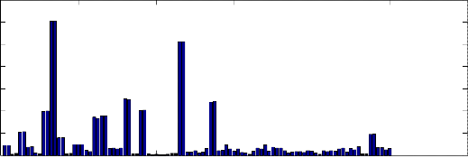
3.5 x 10
4 diff. betw een max and min signal, 30 min before PAF
3
2.5
2
1.5
1
0.5
0
0 20 40 60 80 100 120
records(1-50 normal, 50-100 PAF)
Fig. 8 Histogram of the signal difference between (max. and min.) signal for all records.
2.4 Support Vector Machine (SVM).
The SVM is a discriminative classifier formally defined by margins) between the two classes of the training samples a separating hyperplane (the plane with maximum within the feature space by focusing on the training cases
IJSER © 2013 http://www.ijser.org
International Journal of Scientific & Engineering Research, Volume 4, Issue 12, December-2013 74
ISSN 2229-5518
placed at the edge of the class descriptors so not only an optimal hyperplane is fitted, but also training samples are effectively used. In that way high classification accuracy is achieved with small training sets [12].
In soft margin classification, the SVM algorithm can be summarized as the following optimization problem: given a training set (xi, yi), i=1,2,..,n
σ (kernel width) : is the distance between closest
points with different classifications
C, σ were experimentally defined to achieve the best
classification result.
3 RESULTS AND DISCUSSION
To evaluate the performance of the proposed
min[1 WTW + C ∑n
ξ ] for all {(xi ,yi)}
method during 30-min preceding the (PAF), we

2 i=1 i
Subjected to: yi (wT Φ(xi )+ b) ≥ 1- ξ and ξi ≥ 0 for all i
(2)
divide 30-min period into 6 intervals, 5-min each.
Four measures are used as follows:
TP
Where : Φ(x) is a nonlinear function that maps x into a
Sensitivity(%)=
TP+FN

100 (11)
higher dimensional space.
W, b, and ξ are the weight vector, bias, and slack variable
TN

Specificity (%) =
TN+FP
100 (12)
TP
respectively. C is a constant determined a priori.

PositivePredicitivity(%)=
TP+FP
100 (13)
Parameter C can be viewed as a way to control over fitting. Most “important” training points are support vectors; they define the hyperplane. Quadratic
TP+TN

Accuracy=
TP+TN+FP+FN
Where:
100 (14)
optimization algorithms can identify which training
points xi are support vectors with non-zero Lagrangian
multipliers αi. By constructing a Lagrangian and
transforming it into a dual maximization of the function
Q(α), defined as follows:
max Q(α) =Σαi - ½ΣΣ αi αj yi yj K(xi, xj)
TP: True Positive, when an object having (PAF) is classified correctly.
TN: True Negative when a normal object is classified correctly.
FN: False Negative when an object having (PAF) is classified as normal incorrectly
FP: False Positive when a normal person is classified
Subject to: ∑n
αi yi = 0; 0 ≤ αi
≤ C, for i= 1, 2, …,n
(3)
as having PAF incorrectly
To optimize the learning cost and the
Where K(xi, xj) = φ(xi)Tφ(xj) is the kernel function and αi
classification performance, the SVM classifier
IJSER
is vector of non negative Lagrange multipliers. The kernel
function plays the role of the dot product in the feature
space.
Suppose that the optimum values of the Lagrange
multipliers are denoted α0, it is then to determine the
corresponding optimum value of the linear weight vector wo and the optimal hyperplane as in (4) and (5), respectively:
wo = ∑n 1 αo,i y ϕ(x ) (4)
i= i i
parameters, kernel width σ and regularization constant C, must be chosen effectively [12]. So we chose the parameters σ and C as 10 and 1 respectively.
To evaluate the performance of the proposed
classifier (SVM), we used 60 records (30 n and 30 p)
for training and 40 records (20 n and 20 p) for testing. The four previously mentioned measures are calculated in each 5-min interval. The experiments were repeated 5 trials. In each trial a different set of randomly shuffled samples is done and the
∑n 1 αo,i yi K�x , x � + b (5)
i= i j
The solution is
significant results were tabulated in Table 2
f(x)=sign (∑n
αo,i y K�x , x � + b) (6)
The result of SVM classifier in training data set
i=1
i i j
- Kernel functions may be one of the following types:
- Linear: K(xi,xj)= xi Txj (7)
- Polynomial of power p: K(xi,xj)= (1+ xi Txj)p (8) Gaussian (radial-basis function network):

2
and testing another data set (when two features) is
illustrated in Fig. 9
We can deduce the following points from
analysis of the obtained results:
• We can predict PAF efficiently even in 30 min
K (x , x ) = exp(−
xi − x j
)
prior to PAF
i j 2σ 2
(9)
• The average percentage of the sensitivity,
- Sigmoid: K(xi,xj)= tanh(β0xi Txj + β1) (10)
In this task, we used radial basis function (RBF) as kernel function where:
specificity, positive predictivity and accuracy are higher during 5-min interval preceding the PAF directly.
• The efficiency of the CWT to allow accurate extraction of features from non-stationary signal like ECG.
Trial 1 |
Period (5min) | Sensitivity (%) | Specificity (%) | Positive predicit. | Accuracy (%) |
IJSER © 2013 http://www.ijser.org
International Journal of Scientific & Engineering Research, Volume 4, Issue 12, December-2013 75
ISSN 2229-5518
IJSER
Table 2: Performance evaluation in 5 Trials and the average through 6 intervals in each trial
IJSER © 2013 http://www.ijser.org
International Journal of Scientific & Engineering Research, Volume 4, Issue 12, December-2013 76
ISSN 2229-5518
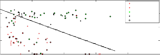
2000
1500
n (training)
n (classified)
p (training)
p (classified) Support Vectors
1000
500
0
0 50 100 150 200 250
Fig. 9: SVM training and classification results
Table 3 Comparative results in the literature
Method | Literature | Sensitivity (%) | Specificity (%) |
HRV | Hariton Costin, et al., 2013 [10] | 84.51 | 83.93 |
MV | Hariton Costin, et al., 2013 [10] | 87.32 | 87.5 |
HRV+MV | Hariton Costin, et al., 2013 [10] | 89.44 | 89.29 |
K-nearest neighbor algorithm | M. Panusittikorn, et al., 2010 [16] | 71.0 | 65.0 |
Proposed method | Ashraf, Hedi, 2013 | 94.0 | 94.0 |
4 CONCLUSION
An efficient method in predicting PAF is
• Robustness of (SVM) classifier to handle large
feature spaces.
• Features like sigmean, sigstd, sigdiff, RRno, RRdiff Ramp and QRSmean enhance the SVM to distinguish between normal ECG record and PAF ECG record
The comparison between the obtained results and other results, in the same field, in the literature [10,
16]
is shown in Table 3
introduced in this task. We extract 11 features from 100 ECG recorded signals of 'afpdp' database with the aid of CWT, to allow accurate extraction of feature from non-stationary signal like ECG, and a Support Vector Machines (SVM) to classify the patterns inherent in the features extracted. The obtained results show the efficiency of the proposed method in predicting the onset of PAF. The average personage of sensitivity, specificity, positive predictivity and accuracy are 94%, 94%, 94.36%, and 94% respectively, and these values overpass the obtained results in the literature
REFERENCES
IJSER © 2013 http://www.ijser.org
International Journal of Scientific & Engineering Research, Volume 4, Issue 12, December-2013 77
ISSN 2229-5518
[1] Poli S., Barbaro V., Bartolini P., Calcagnini G., Censi F., Prediction of Atrial Fibrillation from Surface ECG: Review of Methods and Algorithms. Ann I-st Super Sanità, 39, 2, 195−203, 2003.
[2] Bollmann A., Husser D., Mainardi L. et al., Analysis of Surface Electrocardiograms in Atrial Fibrillation: Techniques, Research, and Clinical Applications. Europace, 8, 911–926, 2006.
[3] Chiarugi F., New Developments in the Automatic Analysis of the Surface ECG: the Case of Atrial Fibrillation. Hellenic J. of Cardiology, 49, 207−221,
2008.
[4] Sörnmo L., Stridh M., Husser D., Bollmann A., Bertil Ollsen S., Analysis of Atrial Fibrillation: from Electrocardiogram Signal Processing to Clinical Management. Phil. Trans. of the Royal Society, A,
367, 235−253, 2009.
[5] S.Karpagachelvi, et al., ECG Feature Techniques- A Survey Approach. International Journal of Computer Science and Information Security, 8, 1, 76-80, 2010.
[6] Moody G.B., Goldberger A.L., McClennen S., Swiryn
Institutului Politehnic din Iaşi Tome LIX (LXIII) Fasc.
1, 2013
[11] Graja S., Boucher J.M., SVM Classification of Patients Prone to Atrial Fibrillation. WISP 2005, IEEE Int. Symp. on Intelligent Signal Proc., University of Algarve, Faro, Portugal, 370−374,
2005.
[12] Maryam, Hassan, Detection of Atrial Fibrillation Episodes using SVM. 30th Annual International IEEE EMBS conference, Vancouver, British, Canada, 177-180, 2008.
[13] Argyro, et al., Robustness of Support Vector Machines-based Classification of Heart Rate Signals. Proceeding of the 28th IEEE EMBS Annual International Conference, New York City, USA, 2159-2162, 2006.
[14] Digvijay, et al., Wavelet Aided SVM Analysis of ECG Signals for Cardiac Abnormality Detection. IEEE Indicon conference, Chennai, India, 9-13, 2005.
[15] Erik Zellmer, et al., Highly Accurate ECG Beat
IJSER
S.P., Predicting the Onset of Paroxysmal Atrial
Fibrillation: the Computers in Cardiology Challenge
2001. Computers in Cardiology, 28, 113−116, 2001.
[7] De Chazal P., Heneghan C., Automated Assessment of
Atrial Fibrillation. Computers in Cardiology, 28,
117−120, 2001.
[8] Maier C., Bauch M., Dickhaus H., Screening and Prediction of Paroxysmal Atrial Fibrillation by Analysis of Heart Rate Parameters. Computers in Cardiology, 28, 129−132, 2001.
[9] Thong T., McNames J., Aboy M., Goldstein B., Prediction of Paroxysmal Atrial Fibrillation by Analysis of Atrial Premature Complexes. IEEE Trans. on Biomed. Eng, 51, 4, 561−569, 2004.
[10] Hariton Costin, et al. A New Method for Paroxysmal
Atrial Fibrillation Automatic Detection. Buletinul
Classification based on Continuous Wavelet
Transformation and Multiple Support Vector
Machine Classifiers. IEEE International
Conference, 1-5, 2009
[16] M. Panusittikorn, et al., Prediction of Paroxysmal Atrial Fibrillation Occurrence with Wavelet-based Markers. IEEE International Conference, 342-345, 2010.
[17] A. K. M. Fazlul Haque, et al., Detection of Small Variations of ECG Features Using Wavelet. ARPN Journal of Engineering and Applied Sciences, 4, 6, 2009
IJSER © 2013 http://www.ijser.org