International Journal of Scientific & Engineering Research, Volume 6, Issue 2, February-2015

ISSN 2229-5518

Effect of Intermittent Power Supply on the

German Power System

Ibrahim A. Nassar

Abstract—In Germany due to the continuous high expansion of the intermittent power supply capabilities of wind turbines and photovoltaic systems, the operational modes of thermal generation units will be influenced essentially until 2020 and beyond. The integration of this increasing share of intermitting generation while maintaining the present security level of supply confronts the existing power system with a big challenge. The fundamental problems are that the intermitting generation does not necessarily fit the power demand and is often located far away from the load centers. This results in physical limitations for integration of intermitting generation with regard to the existing infrastructure. Therefore it is has to be lined out that the acceleration time constant is reduced if some conventio nal power plant generators with masses are disconnected and replaced by the intermittent generators while the total nominal power value of the whole system remains constant. On the other hand more immediate acting acceleration power produced by the turbine-generator-systems of the conventional power plants will disappear because of shut down of these plants and related loss of inertia. With the reduction of inertia not only the frequency deviation after disturbances will increase substantially but also with more oscillation occurs and causes reduction of system stability. Therefore, different methods and tools to simulate the power plant scheduling will be presented and illustrated under different scenarios of Renewable Energy Sources (RES) to check whether the system is stable or unstable.

Index Terms— wind, photovoltaic, inertia, oscillation, stability, primary control, Eigenvalues.

——————————  ——————————

121

1 INTRODUCTION

HE potential of Renewable Energy Sources (RES) is enor- mous as they can in principle meet many times the world’s energy demand. Renewable energy sources such
as biomass, wind, solar, hydropower, and geothermal can provide sustainable energy services, based on the use of rou- tinely available, indigenous resources. A transition to renewa- ble-based energy systems is looking increasingly likely as the costs of solar and wind power systems have dropped substan- tially in the past 30 years, and continue to decline, while the price of oil and gas continue to fluctuate [1 and 2].
In fact, fossil fuel and renewable energy prices, social and en- vironmental costs are heading in opposite directions. Fur- thermore, the economic and policy mechanisms needed to support the widespread dissemination and sustainable mar- kets for renewable energy systems have also rapidly evolved. It is becoming clear that future growth in the energy sector is primarily in the new regime of renewable, and to some extent natural gas-based systems, and not in conventional oil and coal sources. Financial markets are awakening to the future growth potential of renewable and other new energy technol- ogies, and this is a likely harbinger of the economic reality of truly competitive renewable energy systems [3].
RES currently supply somewhere between 15% and 20% of world’s total energy demand. A number of scenario studies have investigated the potential contribution of renewable to global energy supplies, indicating that in the second half of the
21st century their contribution might range from the present
figure of nearly 20% to more than 50% with the right policies
in place. The situation in Europe differs from country to coun-
try. Circumstances may also differ between synchronous in-
terconnected systems and island systems. The capacity targets
and the future portfolio of RES depend on the national situa-

————————————————

 Ibrahim A. Nassar, Department of Electrical Power and Machine, Fac- ulty of Engineering, Alazhar University- Cairo, Egypt, PH-

00201005357921. E-mail: ibrahim.nassar@azhar.edu.eg
tion. Nevertheless, the biggest growth potential is for wind energy. The expectations of the European Wind Energy Asso- ciation show an increase from 28.5 GW in 2003 to 180 GW in
2020 [4].

2 DEVELOPMENT OF RENEWABLE ENERGY SOURCES IN

GERMANY

In Germany, the existing electrical generation system is going to be essentially influenced due to the continuously increasing influence of intermittent renewable energy sources. Because of the massive expansion of the total number of wind turbines, especially in the northern part of Germany within the last years, wind power (WP) now plays the most important role concerning the renewable energy sources in Germany [5].
Table 1 shows the installed capacity for renewable energy generation in Germany since 1990; at the end of 2012, the in- stalled capacity of wind turbines amounted to more than
31.315 GW. Besides the photovoltaic (PV) capacities are in- creasing so fast, that at the end of 2012 there was more than
32.643 GW of installed capacity for photovoltaic systems. In
the photovoltaic sector there was an increase of about 209 %
compared to 2009 [6].
Despite of a stepwise reduction of the feed-in tariffs for the
electrical energy produced by photovoltaic systems and wind
turbines in Germany within the next 10 years, current predic- tions yield to about 50 GW of installed capacity for photovol-
taic systems and an installed capacity of wind turbines of more than 51 GW in 2020. This means that there will be prob- ably more than 100 GW of wind and solar power generation installed in Germany by the end of the decade. Therefore, the share of electrical energy produced by these two renewable sources could increase from 12.6% in 2012 to more than 35% in
2020 of the German electrical net energy consumption [7].

IJSER © 2015

http://www.ijser.org

International Journal of Scientific & Engineering Research Volume 6, Issue 2, February-2015

ISSN 2229-5518

122

TABLE 1

INSTALLED CAPACITY FOR RES IN GERMANY SINCE 1990

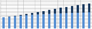
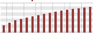
‎0 shows the expected growth of installed capacities of wind turbines (on and offshore) and photovoltaic systems in Ger- many; at the end of 2020, the installed capacity of wind tur- bines and photovoltaic systems amounted to more than 51

GW and 51.7 GW respectively.

Wind onshore Wind offshore

70,0 GW

3 CHALLENGES ON POWER BALANCE AND

FREQUENCY CONTROL

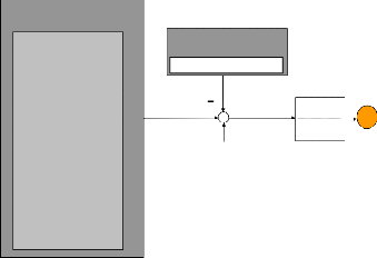
‎0 shows a simplified scheme of the power production

/consumption structure within the model. The crucial item in
this balancing equation is the residual load in each time step
that has to be provided by the dispatchable power generation. At each time the residual load is calculated as the difference
between the power of the consumers and the power produced by the non-dispatchable generation (WP, PV). Therefore as long as the non-dispatchable generation is smaller than the consumed power the residual load is positive. Today this is normally the case all the time because the installed capacities and therefore the maximum simultaneously produced power from these sources is smaller than the network load. The re- sidual load is covered by the dispatchable generation where here the fossil and nuclear plants as well as the pumped stor- age power stations belong to. Hence the dispatchable genera- tion is balancing the intermittent power generation in addition to the consumers demand characteristics.
In future, due to heavily increasing capacities, especially for the wind turbines and photovoltaic systems, the residual load will become negative values in several time periods over the year. In these cases more power is produced than consumed in a single country due to convenient weather conditions in this region. In these cases the power balance would only be ob- served if the dispatchable generation would become negative what respectively means that storage capacities will be in op- eration. But unfortunately the existing storage capacities won’t fit the expected demand in the near future. Hence to observe the active power balance in the system occurring excess power produced by renewable sources has to be curtailed to keep the system stability in some periods in the future if no sufficient transmission line capacities are available to transport the pow- er to other regions.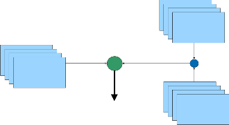

Continuous increase of installed capacities

Non-

dispatchable

60,0 GW

50,0 GW

40,0 GW

Ongoing displacement

Dispatchable

Copperplate model

+ -

generation

Pnon-dispatchable - Residual load

30,0 GW

20,0 GW

10,0 GW

generation

Pdispatchable Presidual

PLoad +

0,0 GW

70,0 GW

60,0 GW

2010 2011 2012 2013 2014 2015 2016 2017 2018 2019 2020 2021 2022 2023 2024 2025

Installed capacity PV

Always Zero, Frequency „Df“ is indicator of power balance

Consumers

No Demand Side Management

50,0 GW

40,0 GW

Fig. 2. A simplified scheme of the power balance of the generation system

30,0 GW

20,0 GW

10,0 GW

0,0 GW

2010 2011 2012 2013 2014 2015 2016 2017 2018 2019 2020 2021 2022 2023 2024 2025

4 DETAILED OVERVIEW OF THE POWER BALANCE OF

GERMAN POWER SYSTEM

Fig. 1. Expected growth of installed capacities of WP and PV in Germany

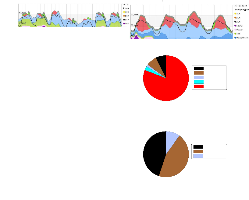
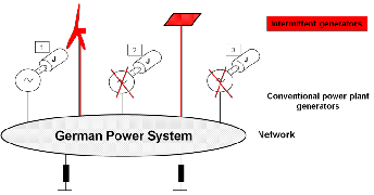
detailed non-linear dynamic model of the German power sys- tem was developed and ‎0 shows the overview of the power

IJSER © 2015

http://www.ijser.org

International Journal of Scientific & Engineering Research Volume 6, Issue 2, February-2015

ISSN 2229-5518

123

balance of German system with all power plants (nuclear power plants (NPP), old and new lignite power plants, old and new hard coal power plants, gas power plants (GPP), old and new combined cycle power plants (CCPP), hydropower Plants (HPP), combined heat and power (CHP)…etc.). The conventional power plants (e.g. thermal, gas, nuclear and hy- dropower plants…etc.) have different transfer functions be- tween frequency and mechanical output power of the tur- bines. All power plants with their primary controllers and loads of German power system are modelled completely in detail. The resulting frequency deviation depends on the pow- er difference, load-damping constant D and the inertia con- stant (TN=2*HN). Where HN is the inertia constant of the sys- tem in seconds and TN is the acceleration time constant of the total network in seconds.

Controlled Power Production with Inertia

TN is calculated by the inertia of the generators and motors, commonly states how much time it takes from standstill to accelerate an inertia that is driven by its nominal torque or power until the nominal rotational speed is reached. Within the electrical energy system the inertia is of vital importance, since only the inertia is able to stabilize the network frequency at an acceptable value in the first moment after a disturbance of the power balance. Normally wind turbines are connected to the system via frequency inverters and photovoltaic sys- tems are always connected via DC/AC converters, so they are mechanically and electrically decoupled from the system and cannot increase the acceleration time constant. Therefore, it has to be lined out that the acceleration time constant is re- duced, if more renewable energy sources (WP and PV) are connected to the system when at the same time the number of conventional power plant generators with masses are dis- placed by these intermittent generators as shown in the ‎0 while the total nominal power value of the whole system re-

Germany

Power Consumption

Consumers Germany

Pload

Pconventional

mains constant.

1

Df

Pintermittent

s.TN  D

Fig. 3. Overview of the power balance of German power system

Any model consists of separate models for power controller, governor and turbine regulator as shown in ‎0. Where Psetpoint is the power setpoint, Δf is the frequency deviation,

Fig. 5. German Power System

The acceleration time constant can be calculated by equation
(1) [8].
Ytref is the set point position governor guide vane, Yt is the

 T .Ρ

J . Ω 2

position governor guide vane and Pm is the mechanical pow-

TN 

i1 Gi Gi

n

and TG 

N (1)

er.

i1 ΡGi  ΡRES Gi

P

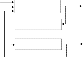
setpoint

Δf

Y

t

Power and Speed Control

Governor

Turbine

Y

tref

P

m

Where TGi is the acceleration time constant for individual units in seconds, PGi is the rated power of an individual Generator in MW, PREF is the intermittent rated power in MW, J is the moment of inertia of the rotor mass in kg-m2 and ΩN is the angular velocity of the mass J in radians per second.
From the moment that a load imbalance is produced in the network to the moment where the grid frequency is fully sta- bilized, several mechanisms take place in the power system during different stages (but in this paper we took only the first two stages), which depend on the duration of the dynamics involved as shown in ‎0. These stages are:
1. Distribution of power impact and inertial response.
2. Primary frequency control or governor response starts within seconds.

Fig. 4. General representation of sub-models

IJSER © 2015

3. Secondary frequency control replaces primary control after minutes by the responsible partner.
4. Tertiary control frees secondary control by re-
http://www.ijser.org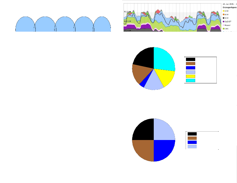

International Journal of Scientific & Engineering Research Volume 6, Issue 2, February-2015

ISSN 2229-5518

124

scheduling generation by the responsible partner

Acceleration Power

of Inertia

of conventional

Power Plants

Primary Control In rotating machines

 3.000 MW ENTSO-E

Secondary Control In rotating machines

2.230 MW GER

Tertiary Control Minute reserve and

“Intra day”

Tertiary Control “Day ahead Planning”

CHP HPP

CCPP/GPP

1st scenario ( 0 % Wind & PV )

22%

27%

17%

15%

Hard coal PPs Lignite PPs GPPs CCGPPS

NNP

HPPs & CHP

4%

16%

Primary reserve

25%

25%

Hard coal PPs Lignite PPs GPPs

CCGPPS

25% 25%

Fig. 9. Contribution of the primary control reserve in the first scenario

cycle gas power plants (CCGPPs). Power plants which are in operation but do not contribute to the primary control are hy- dropower plants (HPPs), combined heat and power plants (CHP) and nuclear power plants (NNPs).

5.2 Second Scenario of Winter 2011 (50% WP and PV)

‎0 shows the second scenario of winter 2011 with 50% intermit- tent renewable energy in operation (wind and photovoltaic). In this scenario, the gas power plants and some of the hard coal power plants are shut down and replaced by wind and photovoltaic power plants (50%). Power plants which are in operation but do not contribute to the primary control are hy- dropower plants, combined heat and power and nuclear pow- er plants.

IJSER © 2015

http://www.ijser.org

International Journal of Scientific & Engineering Research Volume 6, Issue 2, February-2015

I

125

Wind

Solar

2nd scenario ( 47 % Wind & PV )

Wind onshore

3rd scenario ( 81 % Wind & PV )

7%

7%

1%

3%

Hard coal PPs

Lignite PPs CCGPPS HPPs & CHP

Wind & PV

81%

Primary reserve

10%

45%

Hard coal PPs

Lignite PPs

CCGPPS

45%

Fig. 13. Contribution of the primary control reserve in the third scenario

2020. Therefore, ‎0 shows the third scenario of summer 2020 with 81% intermittent renewable energy in operation (wind and photovoltaic). In this scenario the gas and nuclear power plants are shut down and replaced by wind and photovoltaic power plants (80%). Power plants which are in operation but do not contribute to the primary control are hydro power plants and combined heat and power plants.

6 SIMULATION RESULTS

The simulation results have been performed for three scenari- os as explained before. After 5 seconds 700 MW generation loss in German power system, ‎0 shows the frequency response and turbine power for the first scenario (blue line), second scenario (red line) and the third scenario (green line). Due to switching off power plants and replacement by RES to in- crease to 50% and 81% in German system, the existing inertia mass in the grid decreases and deeper frequency deviation (nadir) with more oscillation occurs and shorter oscillation period. With shorter oscillation period, the phase shift be- tween input frequency deviation and output power deviation
produce greater delay as shown in ‎0 ( φ3  φ2 ). As results, for
the first scenario with no intermittent renewable energy in
operation, TN is calculated to 9.9s and the frequency deviation will reach -290 mHz. For the second scenario, the intermittent
renewable energy is increased to 50%, the existing inertia mass

IJSER © 2015

http://www.ijser.org

International Journal of Scientific & Engineering Research Volume 6, Issue 2, February-2015

ISSN 2229-5518

126

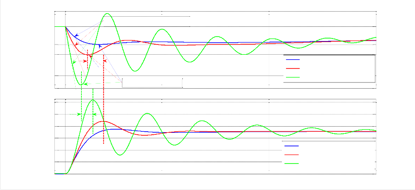
in the grid will decrease, TN is decreased to 5s and the fre- quency deviation will reach -550 mHz with some oscillation occurs. For the third scenario, the intermittent renewable en- ergy is increased to 81%, the existing inertia mass in the grid is
decreased more and TN is decreased to 2s and the frequency deviation is decreased to less than -800 mHz with more oscil- lation occurs. Therefore, some protection devices will operate and switch off some consumers/customers.

Greater decline of initial rate of frequency

50

49.71

49.55 

2

1st scenario, RES 0 %, T

= 9.9s%

49.2

2nd scenario, RES 50 %, T

3rd scenario, RES 81 %, T

= 5s

= 1.98s

N

Lower minimum frequency

49

0 5 50 100 150

1200

1000



3

800

600

400

1st scenario, RES 0 %, T

= 9.9s %

200

2nd scenario, RES 50 %, T

3rd scenario, RES 81 %, T

= 5s

= 1.98s

N

0

0 5 50 100 150

Time in sec.

Fig. 14. Comparison of all scenarios for frequency and turbine power deviation
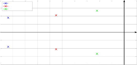
shows the computation of the eigenvalues of German model
Finally, we can conclude that further increase of renewable energy sources in the grid will result in a reduction of the number of connected conventional power plants and this will
for scenarios 1, 2 and 3, as well as the most associated state variables to each eigenvalue, the undamped natural angular
frequency ω (or eigenfrequency) and the damping ratio  .
lead to a reduction of inertia in the grid. This will show a
Let

α jβ be a pair of complex conjugate eigenvalues, the

greater decline of the initial rate of frequency. Lower system

eigenfrequency is defined as ω 

α2  β2

while the
inertia will result in larger and faster frequency deviations
damping is 

  α/

α2  β2 . The damping is positive if

after occurrence of abrupt variations in generation and load.

7 COMPUTATION OF EIGENVALUES FOR GERMAN

POWER SYSTEM

The computations of the eigenvalues have been performed for the German model to make sure that the results from the sim- ulation model are similar. Error! Reference source not found.
the mode is stable (i.e.   0 ). The natural frequency is how
fast the motion oscillates and the damping ratio is how much
amplitude decays per oscillation [9].
As a result, when increasing the RES, the system inertia de-
creases, lead to the eigenfrequency increases and the damping
decreases for scenarios 2 and 3 compared to scenario 1. The
eigenvalues of second and third scenarios approaches more to
unstable region and then the system will oscillate faster.

IJSER © 2015

http://www.ijser.org

International Journal of Scientific & Engineering Research Volume 6, Issue 2, February-2015

ISSN 2229-5518

127

0.4

0.3

0.2

1st scenario, Intermittent 0 %

2nd scenario, Intermittent 50 %

3rd scenario, Intermittent 81 %

T = 9.9s

N

Computation of the Eigenvalues for German power system

T = 5s

N

T = 1.98s

N

0.1

0

stable unstable

-0.1

-0.2

-0.3

-0.4

-0.1 -0.09 -0.08 -0.07 -0.06 -0.05 -0.04 -0.03 -0.02 -0.01 0 0.01

Real Axis

Fig. 15. Computation of eigenvalues for scenarios 1, 2 and 3 for the German Model

8 CONCLUSION

The methods and tools to simulate the power plant scheduling were presented and illustrated by different scenarios of inter- mittent generation. With the reduction of the number of con- ventional power plants during particular time periods the in- ertia time constant of the system will also be reduced. With this reduction not only the frequency deviation after disturb- ances will increase substantially but also the oscillation fre- quency of the so called “Primary Control Oscillation”. So with a fraction of 81% renewable in Germany the deviation after a
700 MW-disturbance will be increased from 390 to 900 mHz, while the oscillation frequency will change from 24 to 43 mHz. In this situation the power system is influenced seriously, be- cause consumers and coupling lines can be tripped simultane- ously which can result in islanding of the system. But also the higher rate of primary control oscillation frequency will re- duce life time of the involved power plants. Finally, we con- clude that a sufficient capacity from conventional generation has to be in the system at any time to keep it stable.

ACKNOWLEDGMENT

This work has been supported by VGB PowerTech e.V. The authors would like to thank all members of the VGB - steering committee and Rostock University, who guided the research project "Influence of Increasing Generation and Consumption Volatility on Reliability of Supply" for their valuable com- ments and advice.

REFERENCES

[1] Herzog, A., Lipman, T. and Kammen, D.: Renewable Energy Sources.

Energy and Resources Group, University of California, Berkeley, U.S.A.

[2] Freris, L. and Infield, D.: Renewable Energy in Power Systems. John

Wiley & Sons, United Kingdom, 2008.

[3] A.K. Akella, R.P. Saini and M.P. Sharma, “Social, economical and envi- ronmental impacts of renewable energy systems,” Renewable Energy, vol.

34, pp. 390-396, March 2009.

[4] EWIS-final report: European Wind Integration Study, 2010.

[5] Bhattacharya, P.: Wind Energy Management. InTech, Croatia, 2011.

[6] Bundesministerium für Umwelt, Naturschutz und Reaktorsicherheit: Erneuerbare Energien in Zahlen. Nationale und internationale Entwicklung, Berlin, 2012.

[7] Weber, H., Ziems, C. and Meinke, S.: Technical Framework Conditions to Integrate High Intermittent Renewable Energy Feed-in in Germany. Wind Energy Management, 2011.

[8] Nassar, I. and Weber, H.: Effects of Increasing Intermittent Generation ‎on the frequency control of the European Power System. 19th IFAC World Congress (IFAC WC 2014), August 24-29, 2014, Cape Town, South Africa, Volume 19/ Part 1, pp. 3134-3139.

[9] Milano, F.: Power System Modelling and Scripting. Power Systems, University of Castilla-La Mancha. Spain,2010

IJSER © 2015

http://www.ijser.org