International Journal of Scientific & Engineering Research,Volume 3, Issue 5, May-2012 1

ISSN 2229-5518

Evaluation of Finite Element Formulation for

One-Dimensional Consolidation

Wan NurFirdaus Wan Hassan, HishamMohamad

Abstract—Consolidation process is defined as the progress of which excess pore water pressure generated by external loading dissipated out of the soil pores and subsequently causing the soil to compress. The ability to predict the dissipation of the excess por e water pressure is important in the assessing the performance of foundations. In this paper, a formulation of Finite Element (FE) method is developed for solving uncoupled consolidation problem and its validity is examined. The basic matrix equations for uncoupling analysis usin g finite elements are derived based on the Galerkin’s weighted residual method. Spatial variables are discretized using the same shape function and a fully implicit scheme is used to discretize the time domain. Using the MATLAB program for writing the FE code, the resu lts are compared with that obtained by classic Terzaghi’s one dimensional consolidation theory. The FE analysis showed good agreement with the

closed form solution.

Index Terms—Consolidation, uncoupled approach,saturated soil, Terzaghi’s theory, Finite Element Method (FEM), implicit.

————————————————————

1 INTRODUCTION

oil made up essentially of soil particle with voids in be- tween. The void generally occupied partly by water and partly by air. Saturated soil is a two phase material consist-
ing of a solid skeleton and water filled voids [1]. When an increment of stress is suddenly applied to an element of satu- rated soil, there is an instantaneous increase in pore pressure and excess pore pressure develops.
The process of consolidation under one-dimensional was first investigated by Terzaghias in[2] and was extended to three dimensional by Biotas in [3]. Both authors agreed that the flow of pore water was governed by Darcy’s law and the response of soil skeleton was elastic.
Finite element formulation based on one-dimensional ide- alization has been established and the numerical characteris- tics have been examined. Desai [4] compared two alternatives for solution of one-dimensional consolidation which used a finer mesh with lower order approximation function and used a coarser mesh with higher order approximating function. They found that, in terms of accuracy, the linear model shows better agreement with the closed form solution compared to the cubic model. An examination of computational time, the cubic model was found to be a about four times longer than for linear model due to the greater degree of connectivity thus increasing the band width of the equation set solution.
The application of the finite element method to the solution of consolidation equation was considered by Sandhu and Wil- son as in [5]. Since then, a number offinite element formula- tionsfor the consolidation of elastic material have appeared.

————————————————

Wan NurFirdaus: Master’s research student, Faculty of Civil Engineering, UniversitiTeknologi Malaysia (UTM), Malaysia. E-mail: fir- sha87@gmail.com

HishamMohamad:Lecturer,Faculty of Civil Engineering, UniversitiTekno-

logi Malaysia (UTM), Malaysia. E-mail: mhisham@utm.my

These include the works ofCarter as in [6], and Menendez as in [7]. Solution techniques for finite element analysis of con- solidation are usually based on first order, implicit integration methods. The backward Euler scheme is widely used in both linear and nonlinear studies. The stability of consolidation analyses has received considerable attention by investigators and many interpolation schemes have been proposed for the time domain.
The stability and accuracy of first order integration schemes has been investigated by Booker and Small as in [1]. They proved that the integration parameter, θ must be less than 0.5 in order for the solution scheme to be unconditionally stable. A fully explicit method is obtained when using θ equal to zero. Vermeer and Verrujit [8] investigated the time steps should not be made too small to avoid oscillation in the pore water pressure and they concluded that a lower limit on the time step, based on the coefficient of consolidation and the mesh size, could reduce the occurrence of oscillatory results. In addition, Abid and Pyrah [9] found that the explicit scheme is not recommended and implicit scheme found to be satisfac- tory and is recommended.
Huang and Griffiths [10] re-examined coupled, uncoupled and the Terzaghi one-dimensional consolidation theories us- ing the finite element method. They concluded, for a layered soil system, combining the coefficient of permeability and coefficient of compressibility into a single coefficient of con- solidation will give wrong excess pore water pressure distri- bution. Recently, Osman [11] found out the uncoupled con- solidation analysis in excellent agreement with the coupled analysis and the uncoupled analysis lead to a relatively sim- pler calculation procedure compared to coupled analysis. Other researcher also concluded that for the case where the flow occurs in one direction when hydraulic conductivity is constant with time, the variation of pore pressure with time calculated from uncoupled analysis becomes identical to that calculated using Terzaghi’s uncoupled analysis [12].
In this paper, a formulation of one dimensional consolida- tion is considered. The finite element is employed to achieve numerical solution, in conjunction with a finite difference

http://www.ijser.org

International Journal of Scientific & Engineering Research,Volume 3, Issue 5, May-2012 2

ISSN 2229-5518

time-stepping algorithm to define the transient nature of the problem.

a' v

p dp

(6)

2 THEORY OF CONSOLIDATION

The theory, which is expressed in mathematical form, becomes

With negative sign ignored. Before any pore pressure dissi- pates, dp = du, so de = du, which can then be substituted into equation (4) to give
the basis for all the studies of consolidation as well as other subjects related to the deformation of the flow of fluids

k 1 e 2 u u

av w z 2 t

(7)
through the porous media. The following assumptions are
essential for the general development of the consolidation
theory as first given by Terzaghi:[13]

The bracketed terms can be defined as the coefficient of con- solidation, or
1. Soil in the consolidating layer is homogenous.
2. Soil is completely saturated (S=100%).

c k 1 e

av w

(8)
3. Compressibility of either water or soil grains is negli- gible.
4. Strains are infinitesimal. An element of dimension dx,
And the coefficient of volume compressibility, (and intro-
ducing the initial in situ void ratio, for e) as

dy, and dz has the same response as one with dimen- mv
sions x, y, and z.

1 e0

a' v

(9)
5. Flow is one-dimensional.
6. Compression is one-dimensional.
7. Darcy’s law is valid (v=ki).
8. Soil properties are constants.
has the units of stress-strain modulus (kPa or Mpa). It is

often referred to as the constrained modulus and is the mod- ulus of deformation, Es. Rewrite in a form suitable for finite element analysis.
9. The void ratio, e vs. pressure, p response is linear. c v
For one-dimensional flow (in the vertical direction or z), the

k(1 e)

av w

w mv

(10)
volumetric flow is defined as

Rewrite Equation (7) as

k h dxdydz dV

z2 dt

(1)

k u m u

w z 2 t

(11)
The element volume is dx dydz and the pore volume is (dx

dydz) [e / (1+e)]. All volume changes V are the pore volume

The solution of Equation (11) is not trivial and uses of Taylor

series expansion. It is as follows:
changes from assumption 3, so the time rate of volume change
as

u 4ui

1 sin 2N
1 z dz e

2N 1 2

H 2

cvt

(12)

dxdydz e dV

(2)
2N 1 H

t e 1 dt

Since the (dx dydz) / (1+e) is the constant volume of solids, Equation (2) can be rewritten as [(dx dydz) / (1+e)] (∂e /∂t). Equating this into Equation (1):

This equation is general and applies for any case of initial

hydrostatic pressure, in a thickness of soil, z and H refers to drainage path. Since the coefficient of consolidation, is constant and time, t is a multiple of H, a dimensionless time

k h e e

z 2 e 1 t

(3)
factor, T can be defined as

c t

T v i

Only a pressure head in excess of the hydrostatic head will H 2
(13)
cause flow (and volume change) and since h = Δu/ Equation
(3) can be rewritten as
The average degree of consolidation as in the following equa- tion:

k 2 u 1 e

(4)

2 N 1 2

8 1 H 2

cvt

1 (14)

w z 2

1 e t

U e

2 2N 1 2
From the slope of the linear part of an arithmetic plot of void
ratio, e or strain, ε versus pressure, p, the coefficient of com-

pressibility, and the compressibility ratio, can be de- fined as

3 FINITE ELEMENT FORMULATION

To derive the basic matrix equations for consolidation, the

a e de

v p dp

(5)
starting point is the differential equation. The governing dif-
ferential equation for consolidation process can be written as

m u k u 0

t w z 2

(15)

http://www.ijser.org

International Journal of Scientific & Engineering Research,Volume 3, Issue 5, May-2012 3

ISSN 2229-5518

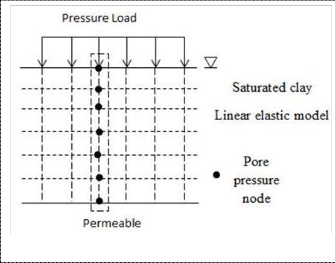
The spatial discretization of the problem is achieved by us- ing linear approximation function as shown in Figure 1. The

u ui

ui 1

clay layer is divided into 20 uniform elements. The element
Equation (19) becomes:
has two nodes with 2 degree of freedom. Since in this paper, the uncoupled approach is considered, the secondary variable

mv N

Nui

Ni 1 dz

k dN dN

uidz 0

(20)
(settlement) will be calculated separately once the primary 0

variable (pore pressure) has been obtained as in [9]. The pore 1

t w dz dz

1 k 0
pressure is linear variation along the element and can be ex-

mv M ui

mv M

ui 1

K ui

(21)
pressed as:

Rearrange the eqution:

u N1u1

N2u2

(16)

1

mv M ui

K ui

mv M

ui 1

(22)

where and denote the nodal pore pressure associated t w t

with the shape function of the element;

where: L is the length of the element,

z z L

dN1 dN1

dN1 dN2

N1 1

, N2 (17)

H H

Stiffness matrix, K

dz dN2

0 dz

dz dN1

dz dN2

dz,

L N N N N

Mass matrix, M

1 1 1

2 dz

N N N N

0 2 1 2 2

Matrix equations of elements have been obtained for the
case of one-dimensional consolidation. Based on that, the pro- gram is coded using MATLAB in this paper.

Fig. 1.Finite element discretization of one-dimensional consolida- tion.

When Equation (16) is substituted into the differential equa- tion of consolidation, the following equation can be obtained.

4 NUMERICAL EXAMPLE

The case is a clay layer of thickness 7m subjected to a vertical pressure of 100kPa and maintained constant with time. Drain- age is allowed from the top and bottom surface. The clay layer is divided into 20 uniform elements. And the time step of =
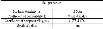
0.05 day was used. The following material properties are as-

TABLE 1

MATERIAL PROPERTIES

m u k

t w

2 N1N2

u1u2 T 0

(18)
Following the standard Galerkin’s weighted residual ap-
proach, a solution of partial differential equation of consolida- tion can be achieved by multiply the whole Equation (11) with shape function of pore pressure and , then integrate it over the element. The need to apply integration by part is important in order to decrease the order of the governing dif- ferential equations. The residuals are set zero, the following equations can be obtained [14].
sumed:
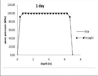
Figure 2(a), 2(b), 2(c), and 2(d), shown a plot of the excess pore pressure with depth from the numerical solution and from Terzaghi’s solution, at four different times after applied

mv N

u dz

k N u

k dN dN

uidz 0

(19)
of loading, i.e. 1 day, 100 days, 365 days and 600 days. The
results show very good agreement between the numerical

0 t w z 0

w dz dz

analysis and the exact solution.
Generally, a finite difference solution to the time integration

has been used. Booker and Small [1] suggested that θ ½ can keep the stability of integration scheme. The implicit time integration (Euler backward) is used and θ 1 is adopted here. Term derivatives of time may be written in finite differ- ence form as:

http://www.ijser.org

International Journal of Scientific & Engineering Research,Volume 3, Issue 5, May-2012 4

ISSN 2229-5518

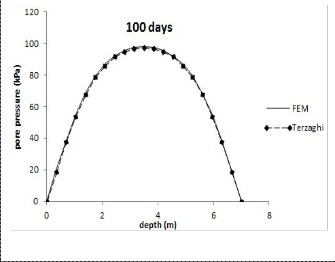
Fig. 2(a).Comparisons of excess pore pressure along depth at time, t =1 day.

Fig. 2(d).Comparisons of excess pore pressure along depth at time, t =600 days.

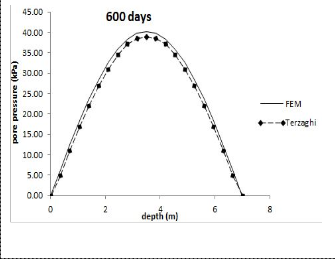
Figure 3 is graph of the average degree of consolidation, U versus the dimensionless time factor, Tv. Similar results of degree of consolidation were obtained from the numerical solution and the exact solution of Terzaghi’s theory.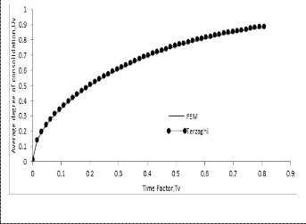

Fig. 2(b).Comparisons of excess pore pressure along depth at time, t =100 days.

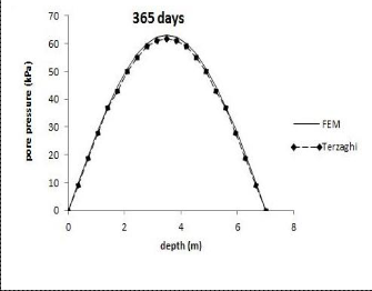
Fig. 3.Average degree of consolidation, U versus time factor, Tv:

comparison between Terzaghi’s exact solution and FEM.

Fig. 2(c).Comparisons of excess pore pressure along depth at time, t =365 days.

5 CONCLUSION

In this study, the problem of the consolidation of an elastic saturated soil was solved with success using finite element method. A formulation consistent with the Terzaghi’s one- dimensional theory has been developed and it has been re- stricted to the case of soils with linear elastic.
The numerical algorithms implemented in this paper are ef-
ficient due to the result which shows a good agreement with the Terzaghi’s exact solution. Further work is currently under- going in order to extend this theory to the analysis of soils with non-elastic behaviour and coupled consolidation ap- proach.

http://www.ijser.org

International Journal of Scientific & Engineering Research,Volume 3, Issue 5, May-2012 5

ISSN 2229-5518

REFERENCES

[1] J.R. Booker and J.C. Small, ‚Finite Element Analysis of Primary and Secondary Consolidation,‛ International Journal Solids Structures, vol.13, pp.137-149, 1977.

[2] K. Terzaghi, ‘Die Berechnung der Durchlassigkeitsziffer des Tones ausdemVerlauf der hydrodynamischenSpannungsersceinungen’, Originally published in 1923 and reprinted in From Theory to Prac- tice in SoilMechanics, John Wiley and Sons, New York, 133-146, 1960.

[3] M.A. Biot, ‚General Theory of Three-Dimensional Consolida-

tion,‛Journal of Applied Physics, vol.12, pp.155-164, Feb 1941.

[4] C.S. Desai and L.D. Johnson, ‚Evaluation of Two Finite Element Formulations for One-Dimensional Consolidation,‛ Computers and Structures, vol.2, pp.469-486, 1972.

[5] R.S. Sandhu and E.L. Wilson, ‚Finite Element Analysis of Flow in Saturated Porous Elastic Media,‛ Journal of Engineering Mechanics Di- vision, ASCE, vol.95, issue 3, pp.641-652, 1969.

[6] J.P. Carter, J.C. Small, and J.R Booker, ‚A Theory of Finite Elastic

Consolidation,‛ International Journal Solids Structures, vol.13,pp. 467-

478, 1977.

[7] C. Menendez, P.J.G. Nieto, F.A. Ortega, and A. Bello, ‚Mathematical Modelling and Study of the Consolidation of an Elastic Saturated Soil with an Incompressible Fluid by FEM,‛ Mathematical and Computer Modelling, vol.49, pp.2002-2018, 2009.

[8] P.A. Vermeer and A. Verruijit, ‚An Accuracy Condition for Consoli-

dation by Finite Elements,‛ International Journal for Numerical and

Analytical Methods in Geomechanics, vol.5, pp.1-14, 1981.

[9] Abid, M.M. and I.C. Pyrah, Guidelines for Using the Finite Element

Method to Predict One-Dimensional. 1988.

[10] J. Huang and D.V. Griffiths, ‚One-Dimensional Consolidation Theo- ries for Layered Soil and Coupled and Uncoupled Solutions by the Finite Element Method,‛ Geotechnique, 2009, doi:

10.1680/geot.08.P.038.

[11] A.S. Osman, ‚Comparison between Coupled and Uncoupled Consol- idation Analysis of a Rigid Sphere in a Porous Elastic Infinite Space‛, Journal of Engineering Mechanics, vol. 136, No. 8, pp.1059-1064, August

2010, doi:10.1061/_ASCE_EM.1943-7889.0000149.

[12] G.C. Sills, ‚Some Conditions under Biot’s Equation of Consolidation Reduced to Terzaghi’s Equation,‛ Geotechnique, vol.25, issue 1, pp.129-132, 1975.

[13] S. Helwany, Applied Soil Mechanics, John Wiley & Sons, Inc., Hobo- ken, New Jersey, pp.123-135, 2007.

[14] J.C. Liu, W.B. Zhao, and J.M. Zai, ‚Research on Seepage Force Influ- ence on One-Dimensional Consolidation,‛ Unsaturated soil, Seepage, and Environmental Geotechnics (GSP 48), pp.203-209, ASCE 2006.

http://www.ijser.org