International Journal of Scientific & Engineering Research, Volume 6, Issue 1, January-2015 690

ISSN 2229-5518

ENERGY BASED ANALYSIS OF MECHANICAL SYSTEM

Oisik Mishra, Sanchari Chakraborty

Abstract — This paper is on Energy based Analysis of Mechanical Systems using Lagrangian and Hamiltonian approach. These approaches can be used to understand the non-linearity and further to control a dynamic system efficiently by using the Kinetic and Potential Energy of the system. Here, we choose an inverted Double Pendulum System as the mechanical system for our analysis. We determine the equations of motions for the double pendulum system using the Lagrangian and Hamiltonian Mechanics and further we implement these concepts to analyse the non-linear properties of the system and further simulate the system in MATLAB.

Keywords — Double pendulum, Dynamics of non-linear system, Energy based control, Inverted double pendulum system, Lagrangian and

Hamiltonian approach, Mechanical system, Non-linear control system.

——————————  ——————————

1 INTRODUCTION

This paper contains the application of Lagrangian and Hamiltonian Mechanics concepts in an Inverted Double Pendulum System to observe its non-linear characteristics. These concepts of Lagrangian and Hamiltonian Mechanics use the Kinetic and Potential Energy of the system. We first determine the equations of motion for the inverted double pendulum system using the concepts of Hamiltonian and Lagrangian Approach and then we determine the state space for the system and we simulate the system in MATLAB to observe the non-linear characteristics of the system. These observations can be used further to design an efficient control system for the inverted double pendulum system from the energy based approach. But this paper is restricted only to the study of the non-linearity of the
system and simulation of the system in MATLAB.

2 LITERATURE REVIEW

In this paper we are modelling the behavior of the system consisting of an Inverted Double Pendulum. We will also calculate the energy in the system. In short, we will model the system using the Lagrangian-Hamiltonian Approach as well as using the SimMechanics toolbox of MATLAB and observe the Non-linear behavior of the system.

2.1 Variables and Parameters

The system will be consisting of two masses connected by weightless bars. The top bar is having length L1 and attached mass m1 . The second bar attached to mass m1 is having length

————————————————

Oisik Mishra is currently pursuing Master of Technology in Energy Systems in University of Petroleum & Energy Studies, India

E-mail: oisik.mishra@stu.upes.ac.in

Sanchari Chakraborty is currently pursuing Bachelor of Technology in Applied Electronics & Instrumentation Engineering in Asansol Engineering College, India

L2 and mass m2 . We can say there are two pendulums, first with mass m1 and length L1 , second with mass m2 and length L2 and having a pivot point O. We will let the angle that the first bar makes with the vertical line drawn down from O be θ1 and that the second bar makes with a vertical line drawn from m1 be θ2 , where counter clockwise angles are positive. If we set this system in xy- plane with O as
origin, we can find the position of the two masses. We will let the x-position of mass m1 as x1 and y- position of mass m1 as y1 . The x and y position of mass m2 will be x2 and y2 . This will give us the variables and parameters correspond to the labels as indicated in fig1.

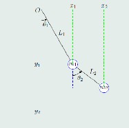
Fig1. Double Pendulum
Hence, the parameters are:
Length of the bar of the first pendulum = L1
Mass at the end of the first pendulum = m1
Length of the bar of the second pendulum = L2
Mass at the end of the second pendulum = m2
The point O is the origin and is where the first pendulum pivots from.
Angle made by the first pendulum and the line of rest = θ1
Angle made by the second pendulum and the line of rest =
θ2
The x-position of m1 = x1
The y-position of m1 = y1

International Journal of Scientific & Engineering Research, Volume 6, Issue 1, January-2015 691

ISSN 2229-5518

The x-position of m2 = x2
The y-position of m2 = y2
We will let that the Kinetic Energy in the system is K and the Potential of Gravitational Energy of the system is P.

2.2 Position of Masses

Equations for the x-position and the y-position of

the ﬁrst mass using trigonometry:

x1 = L1 sin(θ1 ) (1)
y1 = −L1 cos(θ1 ) (2)
To ﬁnd the position of the second mass we will simply add to the position of the ﬁrst mass.
x2 = x1 + L2 sin(θ2 )
energy available to the system caused by the pull of the gravity).
The potential energy is given by:

P = m1 gy1 + m2 gy2

With substitution from the equation (2) and (4), we get,

P = − (m1 + m2 )gL1 cos(θ1 ) − m2 L2 g cos(θ2 ) The kinetic Energy of the system is given by: K= (1/2) m1 (x1 ˙2 + y1 ˙2) + (1/2) m2 (x2 ˙2 + y2 ˙2)

By using equations (9), (10), (11) and (12), we get

K = (1/2 )m1 θ1 ˙2 L1 2 + (1/2)m2 [θ1 ˙2 L1 2 + θ2 ˙2L2 2 + 2 θ1 ˙L1

θ2 ˙L2 cos(θ1 - θ2 )]

2.4 Lagrangian and Hamiltonian Approaches

For this we get,
x2 = L1 sin(θ1 ) + L2 sin(θ2 ) (3)
Similarly for y-position, y2 = y1 − L2 cos(θ2 )
From this we get,
y2 = −L1 cos(θ1 ) − L2 cos(θ2 ) (4)
Differentiating Equations (1),(2),(3) and (4), we get ,
x˙1 = L1 cos(θ1 )θ1 ˙ (5)
y˙1 = L1 sin(θ1 )θ 1 ˙ (6)
x˙2 = L1 cos(θ1 )θ1 ˙ + L2 cos(θ2 )θ 2 ˙ (7)
y˙2 = L1 sin θ1 θ1 ˙ + L 2 sin(θ2 )θ 2 ˙ (8)
Squaring the above equations we get,
x1 ˙2 = L1 2 cos2(θ1 )θ1 ˙2 (9)
y˙1 2 = L1 2 sin2(θ1 )θ1 ˙2 (10)
x2 ˙2 = L1 2 cos2(θ1 )θ1 ˙2 + 2L1 L2 cos(θ1 ) cos(θ2 )θ 1 ˙θ2 ˙ + L 2 2
cos2(θ2 )θ2 ˙2 (11)
The Lagrangian is given by:

Lagrangian = Kinetic Energy – Potential Energy

The Hamiltonian is given by:

Hamiltonian = Kinetic Energy + Potential Energy

3 MATLAB MODEL OF THE SYSTEM

We simulate the Inverted Double Pendulum System in two ways. First we use the Lagrangian-Hamiltonian Approach for modelling and observe the non-linear characteristics of the Angle Position with Time. Secondly, we use the SimMechanics Toolbox of MATLAB for modelling of the physical system (i.e. the mechanical system) of the Inverted Double Pendulum and verified the non-linear characteristics of the system again for the Angle Position with Time. The two models are given below:

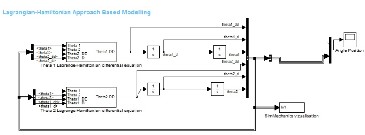
3.1 Modelling in MATLAB using the Lagrangian- Hamiltonian Approach

y2 ˙2 = L1 2 sin2θ1 θ 1 ˙2 + 2L1 L2 sin θ1 sin θ2 θ1 ˙θ 2 ˙ + L2 2
sin2(θ2 )θ2 ˙2.
(12)
Fig2. Modelling of Inverted Double Pendulum System using Lagrangian-Hamiltonian Approach

2.3 Energy of the System

We must observe the energy of the system that consists of two form of energy i.e. Kinetic Energy (the energy of the motion) and the Potential or Gravitational Energy (the

International Journal of Scientific & Engineering Research, Volume 6, Issue 1, January-2015 692

ISSN 2229-5518

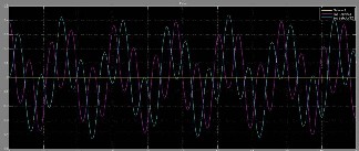
Fig3. Characteristics curves for Angle Position with Time for inverted Double Pendulum System

3.2 Modelling in MATLAB using SimMechanics

Toolbox (Mechanical System Modelling)

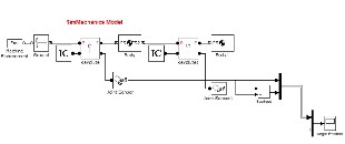
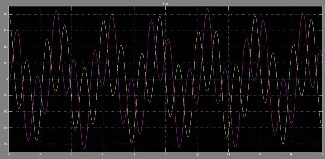
Fig4. Modelling of Inverted Double Pendulum System using SimMechanics Toolbox (Mechanical System Modelling)

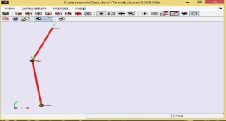
Fig5. Characteristics curves for Angle Position with Time for inverted Double Pendulum System using SimMechanics Toolbox (Mechanical System Modelling)
Fig6. Visualized Model of an Inverted Double Pendulum in
SimMechanics Toolbox of MATLAB

4 OBSERVATIONS

By simulating the Inverted Double Pendulum System by the two methods i.e. using the Lagrangian-Hamiltonian Approach and by using the SimMechanics Toolbox in MATLAB, we obtained the non-linear curves for the behavior of the system i.e. the curves for Angle Position with Time. We found that both the curves obtained for both the methods are similar.

5 CONCLUSIONS

By simulating the system in MATLAB using the Lagrangian-Hamiltonian Approach and the SimMechanics Toolbox (i.e. the Mechanical Modelling) of the Inverted Double Pendulum System, we observed the similar behavior of the Angle Position with Time curves i.e. we observed the similar non-linearity properties of the system.
(It can be seen from the above two graphs obtained). Hence,
the Lagrangian-Hamiltonian Approach or the Energy based
Approach for the study of the system is applicable for the analysis of a Mechanical System.
This method can be further used to study and analyse the mechanical systems and is also helpful for designing an efficient control system for the system.

6 REFERENCES

[1] G. Baker and J.Gollub. Chaotic Dynamics. Oxford
University Press, Oxford, 1990.
[2] L. baker, Gregory and A. Blackburn, James. The Pendulum A Case Study In Physics, Oxford University, Oxford, 2005.
[3] Ohlhoff and P. Richter. Forces in the double pendulum. Z
Angew Math Mech, 22:517– 534, 2006.
[4] Wojciech Szuminski, Dynamics of Multiple
Pendula.
[5] A Double Pendulum, Josh Altic.
[6] Viktor. Prasolov and Yuri Solovyev. Elliptic functions and eliptic integrals. American Mathematical Society, USA, 1997.
[7] Edward Ott. Chaos w układach dynamicznych.
Wydawnictwo Naukowo- Techniczne, Warszawa,
1997.

International Journal of Scientific & Engineering Research, Volume 6, Issue 1, January-2015 693

ISSN 2229-5518