International Journal of Scientific & Engineering Research, Volume 5, Issue 5, May-2014 48

ISSN 2229-5518

Dimensional Analysis Relationships of Geometry Hydraulic Properties For Meandering River in Al Abbasia Reach in Euphrates River

Asst. Prof. Dr. Mohammed Shaker Mahmood, Asst. Prof. Dr. Kareem R. Almurshedi, Zaid Nori Hashim.

Abstract— Most of the hydraulic geometry relationships derived under premises that there are direct or indirect relation, at least statistically, be- tween meander geometry characteristics and some hydraulic variables as discharge and velocity. The authors, based on-a-site investigation on Al- Abbasia reach, in the middle of the Euphrates river, Najaf governorate, developed power functions (four models). The study-reach is about six kilome- ters, it is divided into twenty one cross-sections. These sections represent the meanders and bends in the reach. The recent work is to develop models depending on dimensional analysis and Buckingham Pi theorem. These models are correlate the river width and mean depth with other geometry and hydraulic characteristics. The statistical comparison of the different methods illustrate that the method of dimensional analysis gives higher results in width model comparing with method of power function and lower in mean depth, but acceptable.

Index Terms— Euphrates, Al Abbasia, Najaf; Dimensional Analysis, River Geometry, River Hydraulics, River Meandering, River flow.

——————————  ——————————

1 INTRODUCTION

HE first step in modeling of any physical phenomena is the identification of the relevant variables, and then relat- ing these variables via known physical laws, and one of
the most powerful modeling methods is dimensional analysis. Dimensional analysis is a method for reducing the number and complexity of variables which affect a given physical phenomenon, by using a sort of compacting technique (Frank,1997).[1]
Hydraulic - geometry parameters include width, depth, cross sectional area, and meander length, and other hydraulic vari- ables such as mean slope, friction, and mean velocity which depends on many factors like discharge, and type of bed ma- terial (Singh, 2003).[2]
Most of the hydraulic geometry relationships derived under premises that there are direct or indirect relation, at least sta- tistically, between meander geometry characteristics and some hydraulic variables as discharge and velocity. The mathemati- cal and statistical methods that define these relations begin- ning in growing since (1953). Meandering river and Hydraulic geometry has been one of the most explored and investigated topics in hydraulic engineering. No less than Albert Einstein postulated in 1926 a theory explaining the process of meander- ing on the basis of simple physical laws. Since then under- standing of the process has traversed from simple physics to equilibrium and geomorphic theories on one hand and from empiricism to complex mathematical modelling on the other, and yet without a final word as to-
why and how rivers meander. The real impetus toward for-

————————————————

• Asst. Prof. Dr. Mohammed Shaker Mahmood, Civil Engineering University of Kufa/Faculty of Engineering Najaf, Iraq E- mail: mohammedsh.alshakarchi@uokufa.edu.iq

• Asst. Prof. Dr. Kareem R. Almurshedi, Civil Engineering

University of Kufa/Faculty of Engineering Najaf, Iraq E-

mail: kareem_radhi@yahoo.com

• Zaid Nori Hashim. Civil Engineering University of Kufa/Faculty of Engineer- ing Najaf, Iraq E-mail: zaidnh.enllp@uokufa.edu.iq

mulating a theory of hydraulic geometry was provided by the work of and Maddock (1953). A number of theories have since
been proposed. All theories, however, assume that the river
flow is steady and uniform and the river tends to attain a state
of equilibrium or quasi-equilibrium. The differences are due to
the differences in hydraulic mechanisms that the theories em-
ploy to explain the attainment of equilibrium by the river.
Generally, all the theories can explain how the meandering rivers continue to meander but fail to explain how meanders initiate. Next one exhibits primal theories in hydraulic geome- try, (Singh, 2003).[2]
One of the key steps in the process of mathematical modeling is to determine the relationship between the variables. Con- sidering the dimensions of those quantities can be useful when determining such relationship. Dimensional analysis is a method for helping determine how variables are related and for simplifying a mathematical model. Dimensional analysis alone does not give the exact form of an equation, but it can lead to a significant reduction of the number of variables. It is based on two assumptions:
1. Physical quantities have dimensions (fundamental are mass
M, length L, and time T). Any physical quantity has a dimen-
sion which is a product of powers of the basic dimensions M,
L and T;
2. Physical laws are unaltered when changing the units meas-
uring the dimensions.
Units must be taken into consideration when collecting the
data as well as when making the list of factors impacting the
model and when testing the model. You must check that all
the equations in a model are dimensionally consistent. Nalder,
G., 1997 [3]
Buckingham Pi theorem is a procedure for determining di- mensionless groups from the variables in the problem. The Buckingham Pi Theorem puts the ‘method of dimensions’ first proposed by Lord Rayleigh in his book “The Theory of
Sound” (1877) on a solid theoretical basis, and is based on

IJSER © 2014 http://www.ijser.org

International Journal of Scientific & Engineering Research, Volume 5, Issue 5, May-2014 49

ISSN 2229-5518

ideas of matrix algebra and concept of the ‘rank’ of non-square matrices which you may see in math classes. Although it is credited to E. Buckingham (1914), in fact, White points out that the theorem has also appeared earlier in independent publica- tions by A. Vaschy (1892) and D. Riabouchinsky (1911).[4]
The recent paper focuses on developing a dimensional analy- sis models for width (W) and mean depth (Dm ) to link the dif- ferent geometric and hydraulic characteristics of the river me- anders in the selected river reach.

2 PROBLEM DEFINITION

The authors were developed power function models for the hydraulic geometry in the selected reach (4 models) then were compared with other power functions models in previous studies. This work was published in a paper.[5] Using the di- mensional analysis with Buckingham Pi theorem, the authors developed another multi-variables models for predicting the hydraulic geometry in the same selected reach.

3 SELECTION OF THE REACH

Al-Abbasia reach along the middle part of the Euphrates river was selected to investigate the different geometry hydraulic characteristics. This region is approximately (6000 m) located between Latitudes (32.04°- 32.03°) and Longitudes (44.26°-
44.29°). This selected reach was divided into 21 sections to perform the field work which included measurement of the hydraulic characteristics of the river sections and longitudinal slopes of the stream and soil sampling. Plate (1) shows the selected sections.

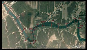
Plate (1): The Selected Reach and Sections.

4 MODELING

4.1 Dimensional Variables

A dimensional analysis of the problem will provide an evalua- tion in non-dimensional terms which will be completely gen- eral. A study of the conditions of flow reveals the problem to be a consideration of the following variables :
1. Variables describing geometry of channels.(X)
- Width of water surface, W
- Mean depth of flow in channel, Dm
2. Variables of flow properties.
- Discharge, Q
3. Variables of fluid properties.
- Mass density of water, ρ
- Kinematic viscosity of water, ν
4. Variables of sediment properties.
- Mean size of bed material, d50
- Specific Gravity Gs
5. Variables of flow production.
- Acceleration due to gravity, g
- Main slope of stream, S

4.2 Data Limitations

Table (1) lists the limitations of the different characteristics of the selected reach (Al-Abbasia) in Euphrates river to perform the analysis in order to produce models for width (W) and mean depth (Dm ). These characteristics were including dis- charge (Q), velocity (V), area of cross-sections (A), width of water surface (W), mean depth (Dm ), max. depth (Dmax ), Main channel slopes (S), mean size of bed material (d50 ), specific gravity (Gs), and viscosity (ν).
Table (1):
Limitations of The Characteristics In Al-Abbasia Reach.

Many parameters as (Ground acceleration, the density of wa- ter and others) were considered fixed within this analysis ei- ther because they are Low changes or that the change does not affect the results, therefore them fixed to facilitate the calcula- tions and comparison. finally, steady flow assumed for analy- sis operations in this research.

4.3 Modeling Procedure

If the geometry of channel parameters are taken to be the de- pendent variable, and the symbol X has been adopted to signi- fy the entry of any one of dependent variable then :
X= Ø( Q ,Gs, d50 ,ρ , ν , g , S ) … (1)
ʄ( X , Q , Gs , d50 , ρ , ν , g , S) = constant … (2)
Where:
Q : Discharge of water.
Gs : Specific gravity .

dR50R : Mean size of particle .

IJSER © 2014 http://www.ijser.org

International Journal of Scientific & Engineering Research, Volume 5, Issue 5, May-2014 50

ISSN 2229-5518

ρ : Density of water.

ЛR5R= Q

a5 .

b5

R50 R

. ρc5

a5

. X … (21)
ν : Viscosity of water.
[M° L° T° ] = � L

b5 c5

� �
g : Acceleration due to gravity .
S : Main slope of river.
For M: 0=c5c5=0

T−1 � �1

L3 �

[L] … (22)
The number of primary dimensions involved is (3), i.e., m=3 (M, L, T). The number of variable is (8), as in Table (1), i. e.,
L: 0=3a5+b5-3c5 +1  b5= - 3a5 -1
T: 0= -1a5 a5=0  b5= -1

ЛR5R =

d50

… (23)
n=8 Therefore, the number of Л- terms 8-3=5, thus:
F{Л1 , Л 2 , Л3 , Л4 , Л5 }= constant ….(3) Now taking Gs , g and ρ repeating variables:
Л1 = Q a1 . d50 b1 . ρc1 . g … (4) Л2 = Q a2 . d50 b2 . ρc2 . Gs … (5) Л3 = Q a3 . d50 b3 . ρc3 . ν … (6)
Table (2) illustrates the summary of the expressions for each
Pi.
Table (2): Expressions for each Pi.



Q
Then relationships can be expressed as following :
Л4 = Q a4 . d50 b4 . ρc4 . S … (7)

X

d50

𝑔 d505

𝑄2

),( 𝐺𝐺 ),(

𝑄

),( S)] … (24)

Л5 = Q a5 . d50 b5 . ρc5 . X … (8)
Table (2): Primary Dimensions for Each Variables.
The following procedure was followed to reduce the number of π-terms:

ν d50

Q 4

ЛR3R/ ЛR1R = ЛR6R = ( g d505 ) = (ν Q/ gd50 ) … (25)

Q2

Thus the functional relationship becomes:
The exponents can be determined under Writing the dimen- sions as in below :

X

d50

X

d50

= ʄ [( ν Q/ gd50

= ʄ [( ν Q/ gd50

4 ),( Gs ),( S)] … (26)

4 ),( Gs ),( S)] … (27)

ЛR1R= Q

a1 . d

b1 . ρc1

. g … (9)
The final form of formula has to be determined from the con-

R50

3 a1 b1 c1

duct of the nonlinear regression analysis on the observed data.

[M° L° T° ] = � L �

T−1

�L�

1

� M �

L3

� L � … (10)

T

W =54× 106 dR50 R(ν Q/ 9.81dR50R 4)-0.23 ( 𝐺𝐺 )-0.01 ( S)0.003 … (28)

Equating exponents of M, L and T
For M: 0=c1c1=0
L: 0=3a1+b1-3c1+1  b1= -3a1-1
T: 0= -1a1-2  a1=-2  b1= 5

g d505

ЛR1R=

Q

… (11)

DR mR =25× 10-4 dR 50R (ν Q/ 9.81dR50R 4)0.6 ( Gs )2.6 ( S)0.017 … (29)

5 VERIFICATION OF THE MODELS

The nonlinear regression analysis was conducted and it was found for width of water surface and mean depth by using the following two models, model (28) for reach width with R2 of

ЛR2R= Q

a2 . d

b2 . ρc2

. Gs … (12)
0.93, and model (29) for reach mean depth with R2 of 0.90.

R50

3 a2 b2 c2

[M° L° T° ] = � L �

T−1

For M: 0=c2c2=0

�L�

1

� M �

L3

[1] … (13)
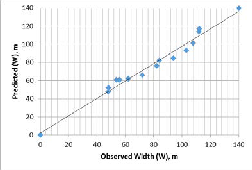
Figure (1) shows the comparison of the model (28) for reach
width (W) corresponding to the observed data. The present multi dependent model illustrates a good correlation of the
L: 0=3a2+b2-3c2  a2= - b2/3
T: 0=-1a2 a2= 0  b2= 0

ЛR2R= Gs … (14)

observed data.
Figure (1): Graphical Comparison of Model (28).

ЛR3R= Q

a3 . d50 b3 c3

R R . ρ

. ν … (15)

a3

[M° L° T° ] = � L �

T−1

b3

� �

1

c3

� �

L3

� L T−1
� … (16)
For M: 0=c3c3=0
L: 0=3a3+b3-3c3+2  b3= - 3a3-2
T: 0=-1a3-1  a3=-1  b3= 1

ν d50

ЛR3R

Q

… (17)

ЛR4R= Q

a4

R50R

b4 . ρc4

. S … (18)

a4

[M° L° T° ] = � L �

T−1

b4

� �

1

c4

� �

L3

[1] … (19)
For M: 0=c4c4=0
L: 0=3a4+b4-3c4  b4= - 3a4
T: 0= -1a4 a4=0  b4= 0

ЛR4R= S … (20)

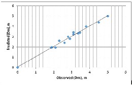
Figure (2) presents the comparison of the model (29) for mean depth of reach (Dm) corresponding to the observed data. The

IJSER © 2014 http://www.ijser.org

International Journal of Scientific & Engineering Research, Volume 5, Issue 5, May-2014 51

ISSN 2229-5518

present multi dependent model demonstrates a good correla- tion of the observed data.
Figure (2): Graphical Comparison of Model (29).

6 VALIDITY OF THE MODELS

It is obtained depending on data collected from 13 different cross-sections. Other of the 21 cross-sections data are used for verification of produced formula by statistical analysis. A F– test was performed to verify the produced models, model (28), and model (29) using the other eight sections in the selected reach. The results of statistical test revealed that there is a good validity of the models, with F–test 0.90 .

7 COMPARISON OF THE MODELS

F-test was used to evaluate the performance of each models (power function versus dimensional analysis) for width and mean depth through giving the extents of error and ac- ceptance with respect to observed values. F-test (or Fisher dis- tribution) has a minimum of 0, but no maximum value (all values are positive). The largest values indicate better agree- ment between measured and calculated values.
Table (3) shows the results of F-test for different predicted models. The dimensional analysis gives good F-test results (0.92 for width and 0.75 for mean depth), while the method of dimensional analysis gives higher results in width model comparing with method of power function and lower in mean depth.
in mean depth.

9 ACKNOWLEDGMENT

The authors wish to thank the staff of Laboratory of Soil at university of Kufa / Faculty of Engineering for their help in laboratory work.

10 REFERENCES

[1] Frank, M.,(1997), "FLUID MECHANICS" University of Rhode Island

Boston, Mc Graw-Hill book company, Fourth Edition.

[2] SINGH, V. P., 2003. ''ON THE THEORIES OF HYDRAULIC GEOMETRY'', International Journal of Sediment Research, Vol. 18, No. 3, pp. 196-218.

[3] Nalder, G., 1997. " ASPECTS OF FLOW IN MEANDERING CHANNELS” IPENZ Transactions, Vol. 24, No. 1/GEN.

[4] Kuntjoro, Bisri, M., and others., 2012. "EMPIRICAL MODEL OF RIVER MEANDERING GEOMETRY CHANGES DUE TO DISCHARGE FLUCTUATION", Journal of Basic and Applied Scientific Research

2(2)1027-1033, ISSN 2090-4304.

[5] Mahmood, Mohammed Shaker, Almurshedi Kareem R., Hashim Zaid N.

''Hydraulic Geometry Relationships for Meadring River in Al Abbasia Reach in Euphrates River'' Vol. 3 Issue 3, March – 2014 International Journal of Engineering Research & Technology (IJERT) ISSN: 2278-0181.

[6] Leopold, L. and Wolman, M. G., 1957. "RIVER CHANNEL PATTERNS: BRAIDED, MEANDERING, AND STRAIGHT" U.S. Geological Survey Professional Paper 282.B

[7] AL-Bahrani, H.Sh., 2012. "A SATELLITE IMAGE MODEL FOR PREDICTING WATER QUALITY INDEX OF EUPHRATES RIVER IN IRAQ” . Ph.D. Thesis, Environmental Engineering Department, University of Baghdad, Baghdad, Iraq.

[8] UN-ESCWA,2013a. (United Nations Economic and Social Commission for Western Asia). "EUPHRATES RIVER BASIN". Inventory of Shared Water Resources in Western Asia. Beirut. Online Version.

[9] UN-ESCWA,2013b. (United Nations Economic and Social Commission for Western Asia). " SHARED TRIBUTARIES OF THE EUPHRATES RIVER ". Inventory of Shared Water Resources in Western Asia. Beirut. Online Version.

[10] MOWR, 2011. Ministry of Water Resources / the National Center for Water Resources Management / Course discharge monitoring (using a device ADCP / M9 .

[11] Harrelson, C., 1994" STREAM CHANNEL REFERENCE SITES: ANILLUSTRATED GUIDE TO FIELD TECHNIQUE" USDA Forest Service General Technical Report RM-245.

Table (3): Values of F-test for Different Models.

Models

Variables

Power Function Dimensional Analysis

Width (W) 0.54 0.92

Mean Depth (D m ) 0.92 0.93

8 CONCLUSION

Dimensional analysis gives two models with good correlation (about 0.9) for both width and mean depth versus the other geometric and hydraulic characteristics. A comparison was made between the models from power function and from di- mensional analysis. The dimensional analysis gives good F- test results (0.92 for width and 0.75 for mean depth), while the method of dimensional analysis gives higher results in width model comparing with method of power function and lower

IJSER © 2014 http://www.ijser.org