Inte rnatio nal Jo urnal o f Sc ie ntific & Eng inee ring Re se arc h Vo lume 3, Issue 3 , Marc h -2012 1
ISSN 2229-5518
Determination of Control Pairing for Higher Order
Multivariable Systems by the use of Multi-Ratios
Ajayi T.O. and I.S.Ogboh
—————————— ——————————
ndustrial processes normally require the control of two or more controlled output variables that relate to production rate, prod-![]()
y(s) ( y1 (s), y2 (s),..., yn (s)) ,
uct quality, safety and environmental concerns. This in turn re-
quires two or more manipulated input variables, thus giving rise to a multi-input, multi-output system (MIMO), or multivariable sys- tem. These multivariable systems are either controlled by a centra- lized controller or by a set of single-input single-output decentra- lized controllers. Decentralized control are more often used for process control applications because it is flexible, simple to design, implement and tune [1]. Decentralized control attempts to control the multivariable system by decomposing it into several single- input-single-output (SISO) control loops. In order to design a de- centralized controller, it is necessary to appropriately pair the input and output variables so as to have minimal interactions from and to the other loops in the closed loop multivariable control system.
yd1
yd2
yd n
u(s) (u1 (s), u2 (s),..., un (s))
u1
u2
Gc(s)
un
y1
y2
G(s)
yn
A lot of interaction measures have been developed to help de- termine the best variable pairing that would achieve minimal inte- raction [2], [3], [4], [5]. The Relative Gain Array, proposed by Bristol in 1966 still has the widest application in industry [6], [7], [8].
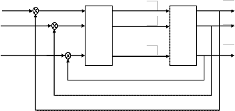
Figure 1. Block diagram of a closed loop mult ivariable control system
and G(s) the trans fer function matrix of the proces s is given by
g11 (s)
![]()
g1n (s)
2.1 The Relative Gain Array (RGA)
![]()
G(s)
Bristol’s Relative Gain Array (RGA) [2] is a well established tool for
gn1 (s)
![]()
gnn (s)
analysis and design of MIMO control systems. Considering the
closed loop multivariable system shown in Figure 1, where the
and the decentralized controller matrix is given by
process to be controlled has an equal number of input; ui, i=1,
2,…,n and output variables; yi, i=1, 2,…,n .
The process transfer function is given by:
gc1( s )
G (s) 0
![]()
0 0
![]()
gc 2( s ) 0
y(s) = G(s)u (s) (1)![]()
c
where![]()
0 0
gcn ( s )
———— ——— ——— ——— ———
where Gc(s) the diagonal matrix of SISO controllers designed based on the diagonal elements of the process transfer func- tion, gii (i = 1…n)
IJSER © 2012
Inte rnatio nal Jo urnal o f Sc ie ntific & Eng inee ring Re se arc h Vo lume 3, Issue 3 , Marc h -2012 2
ISSN 2229-5518
The RGA for a square system is defined as the matrix Λ
such that the element λij is determined as:
and the RGA ,
1
K11K22
K12 K21
![]()
dy
i
du j
all loops open
K K12 K21
K11K22
ij
![]()
dy
![]()
i
du j all loops open except loop u
(2)
while the NI is given by![]()
NI K11 K22 K21 K12
K11 K22
The RGA may be evaluated from the transfer-function matrix of a square multivariable system by doing a Hadamard or Schur product (element-by-element multiplication) of the transfer-function matrix G (s) and the transpose of the inverse
of this matrix, G-T, where
Defining![]()
K 21K12
K11K 22
G (s) (G (s))1 (G (s))T .![]()
The RGA is normally evaluated at steady-state, for which
and rewriting the RGA and NI in terms of ζ, the zeta ratio, gives
G(s) becomes G(0), that is G(s)
and
1
s 0
1
and
NI 1
Λ = G(0) GT (0) and
g(0)
g T (0)
![]()
1 1
ij ij ij
The closer λij is to unity, the better it is to control the ith con- trolled output using the jth manipulated input. Therefore the best control configuration would be one in which the diagonal elements of the RGA are closest to unity, and the rest are clos- est to zero. Skogestad and Morari [10] and Chen et. al[10] and Smith and corripio [11] provide detailed discussions on the use of the RGA.
2.2 The Niederlinski Index [12]
The Niederlinski index determines the best control configuration for a system based on stability analysis. It is defined as:
Both Λ and NI can therefore be said to be functions of ζ
Hence a 2×2 system can be fully characterized by the unirque ratio ξ – the zeta ratio, nd the smaller the value of ξ,
the more perfect is the diagonal pairing However, for higher
order systems, there are many more ratios to be considered.
3.1 The 3×3 System
For a 3×3 system with steady state gain matrix:
NI
![]()
G(0)
n
gii
i 1
(3)
K11
21
K 31
K12
K 22
K 32
K13
23
K 33
A negative value for NI , when all the control loops are closed, implies the system will be integrally unstable for all possible values of controller parameters.
In order to design a decentralized control system for a process, given the transfer function, the RGA is used to obtain a tentative loop pairing, then the NI is used to ascertain the
NI
This can be written fully as,
NI
K
![]()
K11 K22 K33
stability of the closed loop system us ing the recommended RGA pairing, simulation runs are then used to verify if the recommended pairings are suitably stable.
K K K K K K K K K K K K K K K K K K
11 22 33 11 32 23 12 23 31 12 21 33 13 21 32 13 22 31
![]()
K K K
11 22 33
2.3 Defining the zeta ratio for the 2x2 System [1]
Considering a two-input, two-output system whose steady state gain matrix is given by:
(4)
Defining two other variables, Eij, where ij are the various com- binations possible for the 3×3 system (that is 12, 13, and 23) and Dijk.
Kij K ji
![]()
E , and D
Kij K jk Kki
![]()
k11
K G(0)
k12
where,
ij K K ijk K K K
ii jj ii jj kk
k21
k22
Equation (4) can now be rewritten as
IJSER © 2012
Inte rnatio nal Jo urnal o f Sc ie ntific & Eng inee ring Re se arc h Vo lume 3, Issue 3 , Marc h -2012 3
ISSN 2229-5518
NI 1 E23 E12 E13 D123 D213
and the Relative Gain Array, is given by
(5)
Example 1
Using the 2×2 system in [13] in which McAvoy worked on the dy- namic relative gain, DRGA - a modification to the RGA pro- posed by Tung and Edgar [4] and whose transfer function is
1 E23
D123 E12
D213 E13
given by
1 D E
1 E D
E
5e40 s
e4 s
![]()
![]()
NI 213 12 13 123 23
D123
E13
D213
E23
1 E12
G(s) 100s 1 10s 1 .
5e4 s
5e40 s
![]()
Kij cij n
![]()
![]()
10s 1 100s 1
NI Kii
1
where cij is the cofactor of
kij
0.8333 0.1667
The RGA obtained for this system
0.1667 0.8333
Hence a 3x3 system cannot be fully characteriz ed by a unique ratio, as was done for the 2×2 system. It requires the five ratios outlined above. It can further be shown that the number of ratios required for an n ×n system are n! – 1, where n is the dimension of the square gain matrix.
But, as in the case of the 2×2 system, the lower the ratio of the product of the non-diagonal elements in the transfer function matrix to the product of the diagonal ones , the less interactions there are in the system. This was found to be applicable to all square systems regardless of the dimension.
This hypothesis was tested using a MATLAB program based on the algorithm below: (see program in Appendix):
1. Input the matrix dimension, n
2. Input the gain array elements
3. Generate all the possible single loop control configu- rations (n! combinations)
with an NI of 1.2 recommends diagonal pairing, but as is ex- pected due to the dynamic characteristics of the diagonal terms, with time constants and time delays are 10 times slower than the off-diagonal terms, poor closed loop performance was observed by McAvoy et al ([13]. However, as noted in [4] the off-diagonal pairing takes advantage of the fast dynamic characteristics to achieve better closed loop performances. However, the RGA is a steady-state analysis tool which does take the dynamics into consideration.
Using the multi-ratio concept, the program also recom- mends the off diagonal pairing of 1 -2, 2-1 with an NI value of
6.0 and a zeta ratio, ξ = -0.2.
Example 2
Using the model given in [14]for which the transfer function matrix is:
5 2.5e5 s
![]()
![]()
4s 1 (2s 1)(15s 1)
G(s)
4. Evaluate the NI of each of the control configurations
4e
6 s 1
![]()
![]()
5. For the configurations with NI > 0, determine the ξ value (ξ is the ratio of the product of the non-diagonal terms to the product of the diagonal ones in a gain matrix)
6. Sort the viable control configurations in order of in- creasing ξ value (The one with the least value is re- ferred to as the zeta ratio and gives the suitable con- trol configuration).
7. Evaluate the RGA matrix of the this configuration.
The effectiveness of the zeta ratio, ξ, for use in loop pairing in the design of decentralized multi loop controllers is investi- gated.
3.2 Case Examples:
This section tests the hypothesis and shows the effectiveness of using the zeta ratio.
20s 1 3s 1
The RGA obtained for this system
0.3333 0.6667
0.6667 0.3333
with an NI of 3.0 recommends off-diagonal pairing. However, Xiong et. al. [15] in their work on effective RGA (ERGA), using this same model obtained better closed loop performance with diagonal pairing
The program also confirms the result of Xiong in that it re- commends diagonal pairing with an NI value of 1.5 and a zeta ratio, ξ = -0.5.
Example 3
Also using another example used in [15]), a 3 × 3 process whose transfer function is given by
IJSER © 2012
Inte rnatio nal Jo urnal o f Sc ie ntific & Eng inee ring Re se arc h Vo lume 3, Issue 3 , Marc h -2012 4
ISSN 2229-5518
2e s
![]()
10s 1
1.5e
![]()
s 1
s
![]()
s 1
of -2.8601. Using the zeta ratio concept, the program recom- mends the 1-2/2-1/3-3 pairing as optimal with zeta ratio of -
2.021 and an NI = 4.8526.
1.5e e
2e
![]()
![]()
G ( s)
Example 6:
s 1
s 1 10s 1
The model reported in [17] for a complex distillation column
2e
1.5e
with side stream stripper for separating ternary mixtures into![]()
![]()
![]()
3 products is used for the 4 × 4 system. The output variables
s 1 10s 1
and has a relative gain array of
s 1
are the mole fractions of one of the components in each of the
3 phases and the change in temperature (ΔT) while the mani- pulated variables are the reflux ratio, the reboiler heat duty, the stripper heat duty and the stripper flow rate.
The steady state gain matrix obtained is:
4.09
6.36
0.25
0.49
4.17 6.93
0.05 1.53
G(0)
1.73 5.11 4.61
5.49
From which there are two possible recommended pairings 1 -
2/2-1/3-3 and 1-3/2-2/3-1. Using Xiong’s ERGA recommends
1-2/2-1/3-3 as the better of the two pairings but using the zeta
ratio concept recommends the 1 -3/2-2/3-1pairing, which has an NI = 1.5926 and a zeta ratio, ξ = -2.307.
Example 4
Considering a model with one of the elements changed to zero, such that the steady- state gain matrix is given by.
4.19 0 1
11.2 14 0.1 4.49
The program recommends a 1 -2/2-4/3-1/4-3 pairing as op- timal with a positive NI of 46.465 and a zeta value of -3.915 ×
104.
The index is easier to compute than the RGA. It is also easier to analyze, since a single value , and not a matrix is being ana-
G(0) 1
25.96 6.19
lyzed this is acceptable to control practitioners who seem
averse to too much mathematics. A drawback would have
1 1 1
The program failed because of the zero element value since in computing the zeta value, having a zero in the denominator gave an infinite value. To resolve this, a limiting value was substituted to prevent program failure.
The optimal configuration recommended by the program was the diagonal pairing, with RGA given by:
0.8332 | 0 | 0.1668 |
0.0062 | 0.8334 | 0.1604 |
| 0.1666 | 0.6728 |
Example 5
Using the model in [16] whose steady-state gain matrix is giv- en by
been the programme failure when any of the elements in the gain matrix is zero. This difficulty is overcome by replacing the zero value with a limiting value, which for the MATLAB program, the function eps (which is equal to 2.204 x 10 —16) was used
An alternative scheme for determining the optimal control configuration for a multivariable system has been proposed. This method first determines all the control configurations that give a positive NI and then select the one with the lowest zeta ratio, ξ, as the optimal configuration. Comparison with examples based on the RGA or its modification show that the zeta ratio concept, which is much simpler to implement, gives satisfactory result.
0.64
0.21 1.82
G(0) 0.6 1.19
0.34
clear
%Input the dimension of th e square gain matrix and the ma-
0.55
1.12 1.14
trix elements.
%Enter matrix elements ONE AT A TIME ON A row -by-row
and which gave unsatisfactory pairing using the RGA, in that
the RGA recommended pairing returned a negative NI value
and enter 'eps' for elements with zero %value n = input('matrix dimension=')
IJSER © 2012
Inte rnatio nal Jo urnal o f Sc ie ntific & Eng inee ring Re se arc h Vo lume 3, Issue 3 , Marc h -2012 5
ISSN 2229-5518
g=zeros(n,n)
for i=1:n
for j=1:n
g(i,j)=input('gain matrix element')
end
end
%Compute the number of combinations, n -factorial (nf)
nf = 1
for j = 1:n nf = nf*j
end
%Generate all the n-factorial possible gain matrix arrangements in a 3-dimensional array
p = perms(1:n)
M = zeros(n,n,nf)
for k = 1:nf
M(:,:,k) = g(:,p(k,:))
end
%Determine all the PI-control stable configurations by computing
Niederlinski index of each arrangement
for t = 1:nf
a = 1
for k=1:n
a = a*M(k,k,t)
end
ni(t) = det(M(:,:,t))/a
end
%Compute the zeta index for control configurations that have positive Niederlinski indices
for t = 1:nf
if ni(t)>0 a=1
b=1
for i=1:n
for j=1:n
a=a*M(i,j,t) end b=b*M(i,i,t)
end
zeta(t) = a/(b^2)
else ni(t)<0 zeta(t)=NaN end
end
% Compute the RGA for the best configuration c=min(zeta)
r=zeta/c
w=find(r==1)
rga =M(:,:,w).*(inv(M(:,:,w)))'
% Display the suggested control gain matrix configuration
OPTC ONF =M(:,:,W)
[1] Z.X. Zhu and A.Jutan, ―RGA as a measure of integrity for decentra- lized control systems”. Trans. IChemE, Vol. 74, Part A, pp. 35-38, Jan.
1996
[2] E.H. Bristol, ―On a new measure of interaction for mul-
tivariable process control‖. IEEE Trans. Automat. Control, AC-11, pp. 133-134, 1966.
[3] M.F. Witcher and T.J. McAvoy, ― Interacting control sys-
tems: steady state and dynamic measurement of in terac- tion,”. ISA Trans.No. 16, pp. 83 – 90, 1977
[4] L.S. Tung and T.F. Edgar, ―Analysis of control -output in-
teractions in dynamic systems‖. AIChE J., 28, pp. 690-693,
1981
[5] J.P. Gagnepain and D.E Seborg, ―Analysis of process inte-
ractions with applications to muitiloop control system de- sign,‖ Ind. Eng. Chem. Process Des. Dev. 21.pp. 5 -1 1 ,
1982.
[6] F.G. Shinskey, Process Control Systems, McGraw-Hill, New York, pp. 294- 296, 1988.
[7] E.A Wolff and S.Skogestad, ―Operation of integrated
three-product distillation columns,‖ Ind. Eng. Chem. Res. vol. 34, pp. 2094-2103. 1995.
[8] I.E. Hansen, S.B. J.Orgensen, J. Heath, and J.D. Perkins,
―Control structure selection for energy integrated distilla- tion column,” J. Process Control vol. 8 pp. 185-195, 1998.
[9] S. Skogestad and M.Morari, ―Implications of large RGA
elements on control performance,‖ Ind. Eng. Chem. Res., vol. 26, pp. 2323-2330, 1987.
[10] J.Chen, S.J. Freudenberg and C.N. Nett, ―The role of the condition number and the relative gain array in robust- ness analysis,‖ Automatica, vol 30, no. 6, pp 1029 - 1035,
1994.
[11] C.A. Smith and A.B. Corripio, Principles and Practice of Auto- matic Process Control., Wiley, pp. 413-424, 2006
[12] A. Niederlinski, ―A heuristic Approach to the Design of Linear Multivariable Interacting Control Systems,‖ Auto- matica, 7, 691-696, 1971
[13] T.J. McAvoy, Y. Arkun, R.Chen, D. Robinson and P.O.
Schnelle, ―A new approach to defining a dynamic rela- tive gain,‖ Control E ng. Pra ct . vol. 11, pp . 907-914, 2003.
[14] V.J Kariwala, F. Forbes, and E.S. Meadows,―Block relative
gain: Properties and pairing rules,‖ Ind. Eng. Chem. Res., vol. 42, no. 20, pp. 4564–4574, 2003.
[15] Q.Xiong, W.J. Cai, and M.J. He, ―A practical loop pairing
criterion for multivariable processes,‖ J. P roces s Control,
vol. 15 pp. 741-747, 2005.
[16] M.Hovd and S. Skogestad, ―Sequential design of decentra-
lized controllers,‖ Automatica, vol. 30, no. 10, pp. 1601 –
1607, 1994.
[17] S. Skogestad, P. Lundstrom, and E.W. Jacobsen, ―Select-
ing the best Distillation Control Configuration,‖ AIChE J. vol. 36, pp. 753- 761, 1990.
IJSER © 2012