International Journal of Scientific & Engineering Research Volume 2, Issue 4, April-2011 1

ISSN 2229-5518

Designing Aspects of Artificial Neural Network

Controller

Navita Sajwan, Kumar Rajesh

Abstract— In this paper important fundamental steps in applying artificial neural network in the design of intelligent control systems is discussed. Architecture including single layered and multi layered of neural networks are examined for controls applications. The importance of different learning algorithms for both linear and nonlinear neural networks is developed. The problem of generalization of the neural networks in control systems together with some possible solutions are also included.

Index Terms— Artificial, neural network, adaline algorithm, levenberg gradient, forward propagation, backward propagation, weight update algorithm.

1 INTRODUCTION

he field of intelligent controls has become important due to the development in computing speed, power and affordability. Neural network based control
system design has become an important aspect of intelligent control as it can replace mathematical models. It is a distinctive computational paradigm to learn linear or nonlinear mapping from a priori data and knowledge. The models are developed using computer, the control design produces controllers,that can be implemented online.The paper includes both the nonlinear multi-layer feed-forward architecture and the linear single-layer architecture of artificial neural networks for application in control system design. In the nonlinear multi-layer feed- forward case, the two major problems are the long training process and the poor generalization. To
1. Randomly choose the value of weights in the range -1 to 1.
2. While stopping condition is false,follow steps 3.
3. For each bipolar training pair S:t, do step 4-7.
4. Select activations to the input units. X0=1, xi=si(i=1,2…..n).
5. Calculate net input or y.
6. update the bias and weights.
W0=w0(old)+alpha(t-y) Wnew=wi(old)+alpha(t-y)xi.
7. If the largest weight change that occurred in step
3 is smaller than a specified value, stop else

continue.
overcome these problems, a number of data analysis X1 strategies before training and several improvement generalization techniques are used.

2 ARCHITECTURE IN NEURAL NETWOKS

Depending upon the nature of the problems, design of neural network architecture is selected. There are many commonly used neural network architectures for control system applications such as Perceptron Network, Adaline network, feed forward neural network.

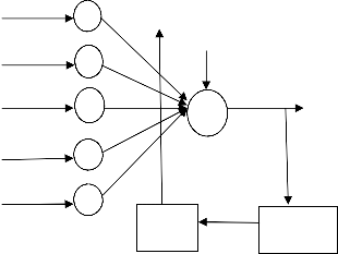
(a)ADALINE Architecture:

X w1

X

X

X

X

0 or 1

y

Wn

Error=t-y t

ADALINE( For ADAptive LINear combiner) is a device Xn
and a new, powerful learning rule called the widrow-
Hoff learning rule this is shown in figure1.The rule
minimized the summed square error during training
involving pattern classification. Early applications of

Adaptive weights

Output error generator

ADALINE and its extension to MADALINE( for many ADALINES) include pattern recognition, weather forecasting and adaptive control

ADALINE algorithm:

Figure 1:ADALINE Neuron Model

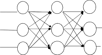
(b)Feed-forward Neural Network Architecture: It is a important architecture due to its non-parametric, non- linear mapping between input and output. Multilayer feed-forward neural networks employing sigoidal hidden unit activations are known as universal approximators.

IJSER © 2011 http://www.ijser.org

International Journal of Scientific & Engineering Research Volume 2, Issue 4, April-2011 2

ISSN 2229-5518

output layers.The output of each node propagates from
the input to the outside side. Nonlinear activation

I2 V21 w13 w21

functions in multiple layers of neurons allows neural a2

b2 c2

network to learn nonlinear and linear relationships between input and output vectors. Each input has an appropriate weighting W.The sum of W and the bias B

V23 V22 w22 Y1

I3 V31 V32 w31 w32 w23

al bm cn

form the input to the transfer function. Any differentiable
activation function f may be used to generate the outputs.
Most commonly used activation function are
purelin f(x)=x, log-sigmoid f(x)=(1+e-x)-1 ,
and tan-sigmoid
f(x)=tan(x/2)=(1-e-x) / (1+e-x)
Hyperbolic tangent(Tan-sigmoid) and logistic(log- sigmoid) functions approximate the signum and step functions,respectively,and yet provide smooth, nonzero derivatives with respect to the input signals. These two activation function called sigmoid functions because there S-shaped curves exhibit smoothness and asymptotic properties. The activation function fh of the hidden units have to be differentiable functions. If fh is linear, one can always collapse the net to a single layer and thus lose the universal approximation/mapping capabilities. Each unit of the output layer is assumed to have the same activation function.

3 BACK PROPAGATION LEARNING

Error correction learning is most commonly used in neural networks. The technique of back propagation, apply error-correction learning to neural network with hidden layers.It also determine the value of the learning rate, I]..Values for I] is restricted such that 0<I]<1.Back propagation requires a perception neural network, (no interlayer or recurrent connection). Each layer must feed sequentially into the next layer.In this paper only the three-layer, A, B, and C are investigated. Feeding into layer a is the input vector I. Thus layer a has L nodes, ai (i=1to L), one node for each input parameter. Layer B, the hidden layer, has m nodes, bj (j =1 to m).L = m = 3; in practice L =I m. Each layer may have a different number of nodes. Layer C, the output layer, has n nodes, ck (k = 1 to n), with one node for each output parameter. The interconnecting weight between the ith node of layer A and the jth node of layer B is denoted as vij, and that between the jth node of layer B and the kth node of layer C is wjk.Each node has an internal threshold value. For layer A, the threshold is TAi, for layer B, TBi, and for layer C, Tck.The Back propagation neural network is shown in figure 2..

V33 w33 Y3

Figure 2: Three-layered artificial neural system
When the network has a group of inputs, the updating of activation values propagates forward from the input neurons, through the hidden layer of neurons to the output neurons that provide the network response. The outputs can be mathematically represented by:
M N
Yp = f(I ((fIXnWnm))*Kmp))
m=-1 n=-1

Yp = The pth output of the network

Xn = The nth input to the network

Wnm = The mth weight factor applied to the nth input

to the network

Kmp = The pth weight factor applied to the mth

output of the hidden layer

F( ) = Transfer function (i.e., sigmoid, etc.)

The ANS becomes a powerful tool that can be used to
solve difficult process control applications
Figure 3 depicts the designing procedure of Artificial
Neural Network Controller.

4 LEARNING ALGORITHMS

A gradient-basedalgorithms necessary in the development of learning algorithms are presented in this section. Learning in neural network is known as learning rule, in which weights of the networks are incrementally adjusted so as to improve a predefined performance measure over time. Learning process is an optimization process, it is a search in the multidimensional parameter (weight) space for solution, Which gradually optimizes an objective(cost)function.

IJSER © 2011 http://www.ijser.org

International Journal of Scientific & Engineering Research Volume 2, Issue 4, April-2011 3

ISSN 2229-5518

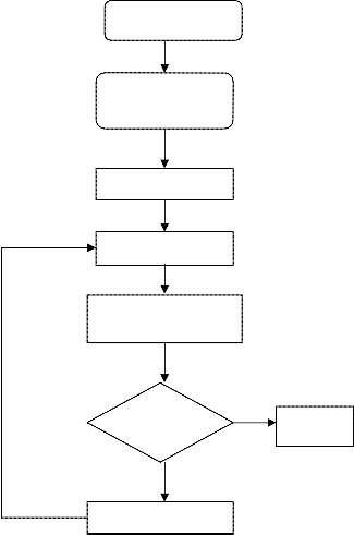
Figure 4: Flow diagram of learning process

Choose ANN methodology

Initialize network parameters(ll, a, no. of neurons), input and output values

Select weight between layers

Calculate network output

5 LEVENBERG GRADIENT BASED METHODS

Gradient based methods searches for minima by
comparing values of the objective function E(8) at
different points.The function is evaluated at points
around the current search point and then look for lower
values. Objective function E(8) is minimized in the adjustable space 8= [81 82,…… 8n] and to find minimum point 8= 8*.A given function E depends on an adjustable parameter 8 with a nonlinear objective function. E(8)=f(81 82,…… 8n) is so complex that an iterative
algorithm is used to search the adjustable parameter
space efficiently. The next point 8new is determined by a step down from the current point 8now in the direction
vector d given as:

Calculate MSE (error between actual output and network output)

If YES

Is

MSE<THRSH

If NO

Change the weights

Network is trained

8next= 8now+I]d
Where I] is some positive step size commonly referred to
as the learning rate.
The principal difference between various descent
algorithms lie in the first procedure for determining
successive directions. After decision is reached, all
algorithms call for movement to a minimum point on the
line determined by the current point 8now and the
direction d.For the second procedure, the optimum step
size can be determined by linear minimization as:

I]*=arg(min(0(I])))

I]>0

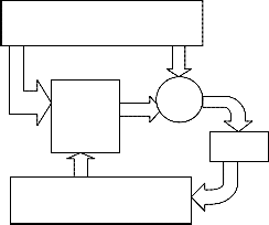
Figure 3: Flow chart for general neural network algorithm

where
0(I])= E(8new+I]d).

TRAINING DATA

NETWORK IN

OUT

Error

+

Target

6 LEVENBERG-MARQUARDT METHOD

The Levenberg_Marquardt algorithm can handle ill- conditioned matrices well, like nonquadratic objective functions. Also, if the Hessian matrix is not positive definite, the Newton direction may point towards a local maximum, or a saddle point. The Hessian can be changed by adding a positive definite matrix AI to H in order to make H positive definite.
Thus,

Weight changes

TRAINING ALGORITHM (OPTIMIZATION METHOD)

COST

Snext = Snow – (H + AI)-1g ,
where I is the identity matrix and H is the Hessian matrix
which is given in terms of Jacobian matrix J as H = JT J.
Levenberg-marquardt is the modification of the Gauss-
Newton algorithm as
Snext = Snow – (JT J)-1 JTr = Snow – (JT J + AI)-1 JT r.
The Levenberg-Marquardt algorithm performs initially
small, but robust steps along the steepest descent
direction, and switches to more efficient quadratic Gauss-

IJSER © 2011 http://www.ijser.org

International Journal of Scientific & Engineering Research Volume 2, Issue 4, April-2011 4

ISSN 2229-5518

Newton steps as the minimum is approached. This method combines the speed of Gauss-Newton with the everywhere convergence of gradient descent, and appears to be fastest for training moderate-sized feedforward neural networks.

7 FORWARD-PROPAGATION AND BACK-

PROPAGATION

During training, a forward pass takes place.The network computes an output based on its current inputs.Each node i computes a weighted ai of its inputs and passes this through a nonlinearity to obtain the node input yi
.The error between actual and desired network outputs is given by
E = 1 (dpi – ypi)2

2 p i
where p indexes the pattern in the training set, I indexes
the output nodes, and dpi and ypi are, respectively, the desired target and actual network output for the error
with respect to the weights is the sum of the individual pattern errors and is given as

dE = dEp = dEp dak

dWij p dWij p,k dak dWij
where the index k represent all outputs nodes. It is convenient to first calculate a value 5i for each node i as

5i = dEp = dEp dyk

dai k dyk dai
which measures the contribution of ai to the error on the current pattern. For simplicity, pattern index p are omitted on yi, ai and other variables in the subsequent equations.
For output nodes, dEp / dak, is obtained directly as
5 = -(dpk - ypk) f (for output node).
The first term in this equation is obtained from error
equation, and the second term which is

dyk = f’ (ak) = f’k

dak
is just the slope of the node nonlinearity as its current value. For hidden nodes, 5i is obtain indirectly as

5i = dEp = dEp dak = 5k dak

dai k dak dai p dai
where the second factor is obtained by noting that if the node I connects directly to node k then dak / dai = f’iwki, otherwise it is zero. Thus,

5i = f’i wk 5k

k
for hidden nodes.5i is a weighted sum of the 5k values of nodes k to which it has connections wki. The way the
nodes are indexed, all delta values can be updated
through the nodes in the reverse order. In layered
networks, all delta values are first evaluated at the output nodes based on the current pattern errors, the hidden values is then evaluated based on the output delta values, and so on backwards to the input layer. Having obtained the node deltas, it is an easy step to find the partial derivatives dEp/dWij with respect to the weights. The second factor is dak/dwij because ak is a linear sum, this is zero if k = i; otherwise
dai

= Xj
dwij
The derivative of pattern error Ep with respect to weight wij is then
dEp

= 5ixj
dwij
First the derivative of the network training error with
respect to the weights are calculated. Then a training algorithm is performed. This procedure is called back- propagation since the error signals are obtained sequentially from the output layer back to the input layer.

8 WEIGHT UPDATE ALGORITHM

The reason for updating the weights is to decrease the error. The weight update relationship is
�wij = I]dEp = I] (dpi – ypi) fixj

dwij
where the learning rate I]>0 is a small positive constant.
Sometimes I] is also called the step size parameter.
The Delta Rule is weight update algorithm in the training of neural networks. The algorithm progresses sequentially layer by layer, updating weights as it goes. The update equation is provided by the gradient descent method as

wij = wij (k+1)- wij(k) = -I] dEp

dwij
dEp = -(dij – ypi)dypi


dwij dwij
for linear output unit, where ypi = wij xi
i and
dypi = xi

dwij

so,
wij = wij (k+1)-wij (k) = I] (dpi – ypi)xi
The adaptation of those weights which connects the input
units and the i th output unit is determined by the
corresponding error ei = 1 (dpi – ypi)2.

IJSER © 2011 http://www.ijser.org

International Journal of Scientific & Engineering Research Volume 2, Issue 4, April-2011 5

ISSN 2229-5518

Training Data Analysis

Two training data analysis methods are: (1)normalizing training set and initializing weights (2)Principal components analysis(speed up the learning process).

9 CONCLUSION

The fundamentals of neural network based control system design are developed in this paper and are applied to intelligent control of the advanced process. Intelligent control can also be used for fast and complex process control problems.

REFERENCES

[1] Rajesh Kumar, Application of artificial neural network in paper industry, A Ph.D thesis, I.I.T.Roorkee, 2009.

[2] S.I.Amari,N.Murata,K.R.Mullar,M.Fincke,H.H.Yang(1997),Asyptotic

Statistical Theory of overtraining and cross validation,IEEE Trans.Neural Networks,8(5),985-993.

[3] C.H.Dagli,M.Akay,O.Ersoy,B.R.Fernandez,A.Smith(1997),Intelligent Engineering Systems Through Artificial Neural Networks,vol.7 of Neural Networks fuzzy logic Data mining evolutionary Programming.

[4] H.Demuth and M.Beale(1997), Neural Networks toolbox user guide,mathworks.

[5] L.Fu, Neural Networks in Computer Intelligence(1994).

[6] M.T.Hang.andM.B.Menhaj(1994),Training feedforward Networks with the Marquardt Algorithm,IEEE Trans. Neural Networks,5(6),989-993.

[7] Hong HelenaMu,Y.P.Kakad,B.G.Sherlock,Application of artificial

Neural Networks in the design of control systems.

IJSER © 2011 http://www.ijser.org