International Journal of Scientific & Engineering Research, Volume 4, Issue 12, December-2013 1556

ISSN 2229-5518

Design and Implementation of a Real-Time Intelligent Controller for a Differential Drive Mobile Robot

Zeyad Yousif Abdoon Al-Shibaany (IEEE Member), Nadia Abd Alzhra Jassar

Abstract— The paper proposes an intelligent kinematic controller to guide a differential drive mobile robot system, which is a nonholonomic differential drive mobile robot, to follow a predefined path. The controller has been designed and implemented by using a Multi-Layer Perceptron MLP neural network. The error back propagation algorithm has been used in order to train the neural network to identify the kinematic model of the differential drive mobile robot. The neural network based controller has been trained offline and then online in order to calculate the required linear and angular velocities to guide the robot throughout the predefined path. The controller has been implemented by using a real-time and FPGA based input/output board, which is fully compatible with LabVIEW 2012 software, and then the controller is being deployed to the mobile robot platform to allow for autonomous navigation. The simulation and experimental results explained and proved that the proposed controller can successfully guide the robot along the required path.

Index Terms— Nonholonomic, Mobile Robot, Neural Network, Real Time, Adaptive Controller, LabVIEW, National Instrument.

——————————  ——————————

1 INTRODUCTION

n general, a mobile robot can be defined as a moveable sys- tem which has the ability to navigate and interact with its
creased significantly [3].
environment by using its IsensorsJand actuatorSs [1]. Wheeled ER
mobile robots have become an interesting area of research
over the last few decades. There are many applications for the
mobile robots such as materials handling, and household ser-
vices.
An intelligent autonomous mobile robot has the ability to
detect and react to its surroundings when it is moving from a
start position to its final position [1]. The detection and reac-
tion abilities can be achieved by using the sensors and actua-
tors of the mobile robot. The two essential components re- quired to read data from the sensors and make decisions based on that sensory data are the processor and control sys- tem. As the requirements of each mission can vary; those four
elements must be presented for any mobile robot to be auton- omous and to function correctly.
By using its sensors, the mobile robot is capable of observ- ing the environment and providing useable data to the proces- sor which in turn uses this data via the control algorithm, to guide the mobile robot throughout the environment [2]. The control system provides the mobile robot with the algorithm required to achieve various missions. The motion control of mobile robot systems has gained considerable attention in the last few years as the applications of mobile robots have in-

————————————————

• Zeyad Yousif Abdoon Al-Shibaany is currently an assistant lecturer in the

Control and Systems Engineering Department – University of Technology

/ Iraq. He obtained his Master degree in Mechatronics engineering from

Newcastle University – United Kingdom with a Distinction and his rank

was the FIRST among all the postgraduate students in 2012. He also had been awarded a prize for the BEST performing Master student in the School

of Mechanical and Systems Engineering – Newcastle University for the ac- ademic year 2011/2012. E-mail: zeyad.al-shibaany@ieee.org.

• Nadia Abd Alzhra Jassar is currently an engineer in the Laser and Optoe-

lectronics Engineering Department – University of Technology / Iraq. She

obtained a B.Sc. degree in Control and Systems Engineering in 2007 from the University of Technology / Iraq. E-mail: nadia_abdalzhra@yahoo.com
Many control strategies have been developed in order to
provide a robust feedback control rule for mobile robot sys-
tems. The control algorithm of any mobile robot depends ei-
ther on the dynamic model or the kinematic model of the mo-
bile robot.
The dynamic controller, sometimes called the torque con- troller depends on the dynamic model of the mobile robot such that the actual velocity of the mobile robot converges to the required velocity, while the main aim of the kinematic con- troller is to output a velocity for the mobile robot in order to reduce the error between the required path and the actual path of the mobile robot system [3].
This paper considers the use of the neural networks be- cause of their learning and adaptation capabilities. Neural network techniques demonstrate very good performance when they have been used in the motion control of mobile robots [3]. Other advantages of a neural network are its ability to provide a very good model of any nonlinear system, and its parallel structure makes the neural network performance fast- er than the performance of other classical artificial intelligence techniques such as a Genetic algorithm. In addition to these, the simple implementation of neural network has made the use of it much easier than other techniques.
A neural network based controller is designed to guide a nonholonomic mobile robot to follow its reference path in [4]. Lyapunov theorem is used to test the stability of the controller and the simulation results show that the controller functions well. A Q-learning neural network based controller is present- ed in [5]. The main purpose of this controller is to enable the mobile robot to determine the optimal path from its initial position to its final goal. The validation and performance of the controller is proved by experimental results as well as by

International Journal of Scientific & Engineering Research, Volume 4, Issue 12, December-2013 1557

ISSN 2229-5518

simulation results. A nonlinear controller is designed and im- plemented based on neural network technique to enable a one wheel mobile robot to be balanced in [6]. The practical results proved that the neural network based controller is much better than classical controllers as the neural network has a very good adaptation feature.

2 THE KINEMATIC MODEL OF THE DIFFERENTIAL DRIVE

MOBILE ROBOT

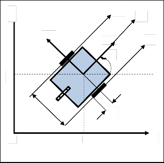
The mobile robot platform shown in fig. 1 has two driving wheels, and one passive wheel which is added for the purpose of stability as the robot requires at least three points of contact with the ground to be statically stable.
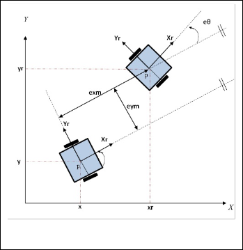
frame is the global (reference) frame which is fixed and denot- ed by X and Y as shown in fig. 1. The posture of the mobile robot is represented by a vector P = [x y θ]T, where x and y are the coordinates of the point p according to the reference frame, and θ is the mobile robot orientation which is the angle be- tween the x axis of the global frame (X) and the x axis of the robot frame (Xr).

Y V2

V

Yr

Xr V1

pIJSER

L r

O x X

Fig. 1. Schematic of the differential drive mobile robot

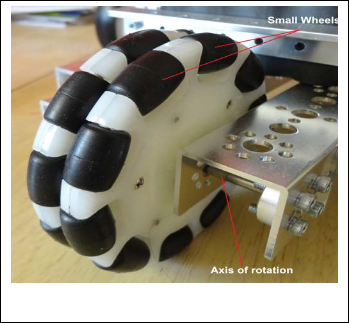
Fig. 2. Omnidirectional wheel of the National Instrument mobile robot

The two driving wheels are free to rotate about their axes of rotation which are coinciding with the y axis of the robot frame (Yr). The linear velocity of the robot (V) is orthogonal to the axis of rotation of the two driving wheels. According to the nonholonomic constraints, the robot is assumed to have no lateral velocity which means the wheels are purely rotating with no slipping [7].

The driving wheels are parallel to each other. The rear passive wheel in this case is an omnidirectional wheel that has small wheels mounted around its circumference. The axis of rotation of these small wheels is perpendicular to the axis of rotation of the omnidirectional wheel in order to eliminate the friction effect when the mobile robot is turning. The small wheels give the omnidirectional wheel an additional degree of freedom. This means the omnidirectional wheel can move forward or backward by rotating around its axis of rotation, and can move laterally when the small wheels are rotating around their axis of rotation. Figure 2 below shows the omnidirection- al wheel of the differential drive mobile robot (National In- strument starter kit) which is used in this paper.
The two driving wheels have the same radius which is denot- ed by r in fig. 1. The distance between the two wheels is de- noted by L. The mobile robot (NI starter kit) is designed and manufactured so that its center of mass is located at point p which is located at the middle of the distance between the two wheels. There are two frames associated with the mobile ro- bot. The first one is the robot frame which is rigidly attached to the mobile robot and denoted by Xr and Yr. The second

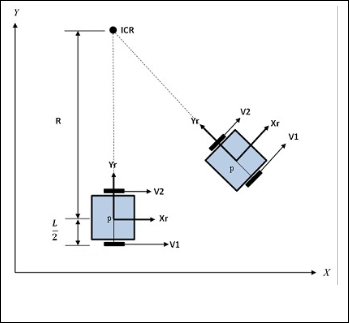
Fig. 3. Mobile Robot Instantenous Radius of Rotation

International Journal of Scientific & Engineering Research, Volume 4, Issue 12, December-2013 1558

ISSN 2229-5518

The two driving wheels of the differential drive mobile robot are moving around the instantaneous center of rotation (ICR) with the same angular velocity (W) at each time instant [8]. The instantaneous center of rotation can be found by drawing a line, which is normal to the driving wheels plane, at a specif- ic time instant then to draw the same line but at different time instant and then the ICR is the point where those two lines meet [9]. This means that the robot is following a circular path with a radius of R and the center point is the ICR [9]. Figure 3 clarifies the process of finding the instantaneous center of rota- tion ICR.
The kinematic model of the differential drive mobile robot system, which is shown in fig. 1, can be derived as follow:

3 STRUCTURE OF THE ADAPTIVE KINEMATIC

CONTROLLER

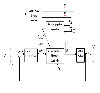
The structure of the adaptive kinematic controller is shown in fig. 4 in the form of a block diagram. The navigation of the mobile robot starts with generating the required trajectory where Pr = [xr yr θr]T is the required pose of the mobile robot. This required pose is used by the inverse kinematic of the mo- bile robot to generate the required linear and angular veloci- ties for the specified trajectory with the required orientation. The error vector is then calculated by comparing the required pose of the mobile robot with the actual pose of the robot. This error is calculated and needs to be transformed into the mobile robot frame by using the transformation matrix R. This error is then used by the controller to produce a control action to force

W (t ) = d θ (t )

V (t ) = W (t ) R(t )

(1)

(2)

the mobile robot to follow the required path.

Now it is easy to calculate the linear velocities of both the right and the left wheels:

V1 (t ) = W (t ) ( R(t ) + 0.5 L)

V2 (t ) = W (t ) ( R(t ) − 0.5 L)

(3) (4)

By solving Eq. 3 and Eq. 4, the ICR can be calculated as:

IJSER

R(t ) = 0.5 L (V2 (t ) +V1 (t ) )

V2 (t ) −V1 (t )

(5)

The linear and angular velocities of the mobile robot can be represented in terms of the linear velocities of the two driving wheels as follow:

V (t ) = V1 (t ) +V2 (t )

W (t ) = V1 (t ) −V2 (t )

(6)

(7)

Fig. 4. Structure of the adaptive neural kinematic controller

In term of the global frame, the kinematic equations of the
mobile robot can be represented as follow:
x(t ) = V (t ) cos (θ (t ))
y (t ) = V (t ) sin (θ (t ))

(8) (9)

The kinematic model of the mobile robot can be written in the form:
θ(t ) = W (t )

(10)

 x(t ) 

cos(θ (t ))

0 V (t ) 

In order to obtain the position and orientation of the mobile

 y (t ) =  sin(θ (t ))

0  

(14)

  

  

robot, it is required to integrate Eq. 8, 9 and 10 as illustrated
below:

θ(t )  0

1 W (t )

x(t ) = x0 + ∫V (t ) cos(θ (t )) dt

y(t ) = y0 + ∫V (t ) sin(θ (t )) dt

(11) (12)

Let (xr , yr) is the required position of the mobile robot, and θr
is the required orientation of the mobile robot, so that the re-
quired posture vector is Pr = [xr yr θr]T. The actual position of
the mobile robot is assumed to be (x,y) and the actual orienta-
tion of the mobile robot is assumed to be θ, so that the actual
posture of the mobile robot is P = [x y θ]T. Then the error
e=[ex ey eθ]T can be calculated in the global frame:

θ (t ) = θ 0 + ∫W (t ) dt

(13)

 ex 

 xr

− x 

   

Where (x0, y0) is the initial position of the mobile robot, and

 ey  =  yr − y

(16)

θ0 is the initial orientation of the mobile robot.

eθ 

θ r − θ 

International Journal of Scientific & Engineering Research, Volume 4, Issue 12, December-2013 1559

ISSN 2229-5518

The error vector e needs to be transferred into the robot frame by using the orthogonal rotation matrix R [10]:

em = R*e (17)

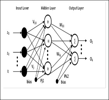
layer [11]. The activation function of the hidden layer nodes in this case is a bipolar sigmoid function. Table 1 explains the abbreviations that have been used in fig. 6. The output of the neural network is calculating as follow:

exm 

 cos(θ (t ))

sin(θ (t ))

0  ex 

Ok = ∑ hnet j ×Wkj + bias × Pk 2

j =1

(19)

eym  = − sin(θ (t ))

cos(θ (t ))

0  ey 

(18)

where hnetj is the output of the hidden layer node j and is be-

  

  

eθm  0

0 1 eθ 

ing calculated as:
Figure 5 illustrates the error transformation from the global

hnet = H (h )

(20)

frame into the robot frame. The error vector em is fed into the controller and then it is the responsibility of the controller to

j j

where:

generate the required linear and angular velocities to reduce
the tracking error.
The controller is designed based on the MLP neural network

h j = ∑ zi

i =1

× V ji

+ bias × Pji

(21)

topology. The adaptive neural kinematic controller learns the behavior of the differential drive mobile robot inverse kine- matics by making use of the neural network’s ability to learn the behavior of nonlinear systems. The identification process includes two stages: offline and online

H (h j ) =

− 1
1 + e h j

(22)

IJSER

Fig. 6. Structure of MLP neural kinematic controller

Fig. 5. Error transformation from global frame into robot frame

TABLE 1

NEURAL NETW ORK PARAMETERS

Figure 6 shows the MLP neural network which consists of three layers: input layer, hidden layer and output layer. The input layer has only three nodes because the input to the con- troller is the error vector which includes the error in robot x coordinate, the error in robot y coordinate and the robot orien- tation error. In the case of the input layer in fig. 6, the input nodes are drawn as solid nodes which mean that those nodes do nothing more than just collect the input of the neural net- work.
The number of nodes in the hidden layer can vary depending on the required performance of the neural network. The suita- ble number of nodes in the hidden layer one can start with is equal to (2n+1) where n is the number of nodes in the input

International Journal of Scientific & Engineering Research, Volume 4, Issue 12, December-2013 1560

ISSN 2229-5518

The error back propagation algorithm technique was used to adjust the weights of the neural network by calculating the error in the output layer and then propagating back this error in order to adjust the weights of the neural network. The weights are adjusted offline and then online.
The neural network learns the exact behavior of the inverse kinematic model of the mobile robot and can then serve as a controller to guide the robot during the trajectory tracking. The weights of the neural kinematic controller can be adjusted during the navigation in case the robot is subjected to an ex- ternal disturbance. Those weights are adjusted by the back propagation algorithm as shown in fig. 4.

4 SIMULATION RESULTS

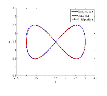
The proposed controller in this paper was designed and tested using MATLAB program before being applied in LabVIEW in order to test the controller functionality before applying it to the real mobile robot platform. In this simulation test, the ro- bot is required to follow a predefined path which is a lemnis- cate. The reason for choosing this path is because it examines all the possible postures of the mobile robot where at each sample the ICR is different. The robot is also required to fol-
low the path with a predefined orientation.
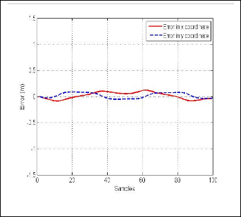
both x and y coordinates.
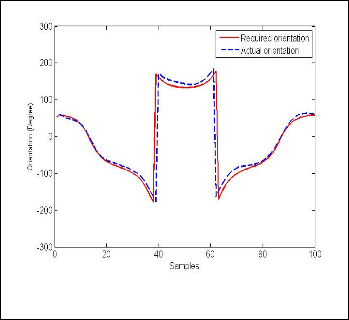
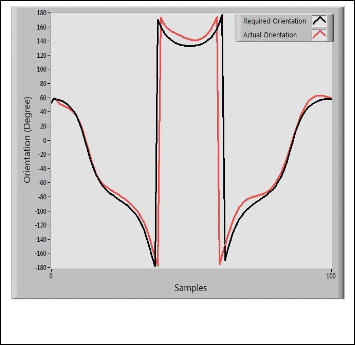
The required orientation of the mobile robot and the simulated
orientation are given in fig. 10. It can be clearly seen that the

robot tracks the reference trajectory.

Fig. 8. The required path and simulated path of the mobile robot

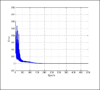
A training set of 100 samples and a learning rate of 0.1 were used to train the neural kinematic controller. The neural kine- matic controller learnt the behavior of the mobile robot model after 2000 epochs with a mean square error equal to 3×10-6 as shown in fig.7.

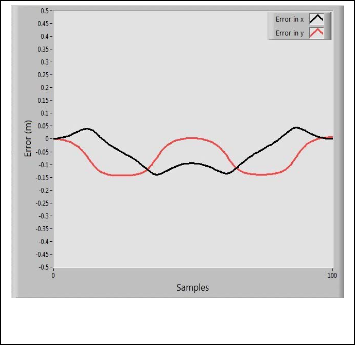
Fig. 9. Error in x and y in the coordinates of the mobile robot

Fig. 7. Error during the identification process

The sampling time in this case is 0.5 second, and the physical parameters of the differential drive mobile robot are: r=5 cm and L=36 cm. Figure 8 shows the required trajectory as well as the simulated path of the mobile robot.
As shown in fig. 8, the robot follows the required path with minimum trajectory tracking error. Figure 9 shows the error in
The simulation results show that the controller functions cor- rectly and prove its ability to guide the robot to follow this complex path with minimum error in the robot position and orientation.

International Journal of Scientific & Engineering Research, Volume 4, Issue 12, December-2013 1561

ISSN 2229-5518

acceptable error in its position. The real orientation of the mo- bile robot is shown in fig. 14 and it can be seen that the robot is in the right orientation with some error because the robot is trying to correct the error in its position which causes an error in the orientation.

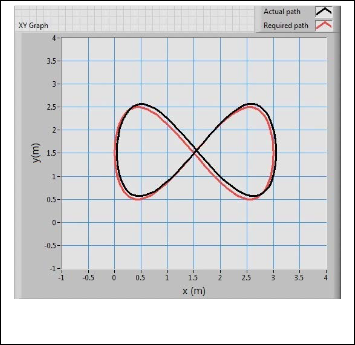
Fig. 10. The required orientation and actual orientation of the mobile robot

5 EXPERIMENTAL RESULTS

The experimental resultsIwere Jobtained by Susing the Na- ER

tional Instrument mobile robot which is shown in fig. 11. This robot is compatible with LabVIEW2011 software and the con- troller is implemented in this software and then deployed to the mobile robot. The robot has two independent driving wheels, and one omnidirectional wheel which is added for the purpose of stability. The robot also has a powerful FPGA based processor with Real-time Input-Output (RIO) board.

Fig. 12. The required path and actual path of the mobile robot (practi-

cal results)

Fig. 13. Error in x and y coordinates of the mobile robot (practical re- sults)

Fig. 11. National Instrument Mobile Robot

Figure 12 shows the required path and the actual (practical) path of the mobile robot. As shown in fig. 12 and fig. 13, the real mobile robot has followed the reference path with some
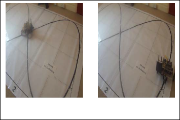
Figure 15 below shows the real mobile robot system while testing the functionality of the controller. The robots followed the predefined trajectory precisely and the controller was working successfully by guiding the robot with minimum er- ror.

International Journal of Scientific & Engineering Research, Volume 4, Issue 12, December-2013 1562

ISSN 2229-5518

Iraq.

Fig. 14. The required path and actual orientation of the mobile robot

(practical results)

REFERENCES

[1] M. T. Chew, S. Demidenko, L. Huang, C. Messom, G. SenGupta, and M. Watts, "Simple Mobile Robots for Introducing into Engineering," presented at the International Instrumentation and Measurement Technology Conference, Singapore, 2009.

[2] Eva. B., J. A. Lopez-Orozco, P. Lanillos, and J. M. Cruz, "Localization of Non-Linearly Modeled Autonomous Mobile Robots Using Out-of- Sequence Measurements," Sensors, vol. 12, pp. 2487-2518,

23/02/2012.

[3] O. Mohareri, Rached Dhaouadi, and Ahmad B. Rad, "Indirect adap- tive tracking control of a nonholonomic mobile robot via neural net- works," Neurocomputing, vol. 88, pp. 54 - 66 2012.

[4] N. A. Martins, D. W. Bertol, W. C. Lombardi, and E. R. de Pieri, "Tra- jectory tracking of a nonholonomic mobile robot: A suggested neural torque controller based on the sliding mode theory,” International Conference on Variable Structure Systems, pp. 384-389, 2008.

[5] V. Ganapathy, S. C. Yun, and H. K. Joe, "Neural Q-Learning Control-

ler for Mobile Robot," IEEE/ASME International Conference on Ad- vanced Intelligent Mechatronics, Vols 1-3, pp. 863-868,2009.

[6] P. K. Kim, J. H. Park, and S. Jung, "Experimental Studies of Balancing

Control for a Disc-Typed Mobile Robot Using a Neural Controller: GYROBO," IEEE International Symposium on Intelligent Control, pp.

1499-1503, 2010.

[7] Y.-T. Wang1, Y.-C. Chen, and M.-C. Lin, "Dynamic Object Tracking Control for a Non-Holonomic Wheeled Autonomous Robot," Tamkang Journal of Science and Engineering, vol. 12, p. 339350, 2009.

[8] S. Han, B. Choi, and J. Lee, "A precise curved motion planning for a differential driving mobile robot," Mechatronics, vol. 18, pp. 486-494, Nov 2008.

[9] R. Siegwart and I. R. Nourbakhsh, “Introduction to autonomous mobile robots,” Second ed.: MIT Press 2011.

[10] J. Ye, "Tracking control for nonholonomic mobile robots: Integrating the analog neural network into the backstepping technique," Neuro- computing, vol. 71, pp. 3373–3378, 23 December 2008.

[11] J. Zurada, “Introduction to Artificial Neural System”: West Publish-

Fig. 15. The real mobile robot during its navigation along the required path.

ing Company, 1992.

6 CONCLUSION

The adaptive neural kinematic controller is proposed in this paper. The proposed controller has been designed and tested in MATLAB where the simulation results prove the function- ality and robustness of the controller. The controller is imple- mented in LabVIEW software and applied to a real mobile robot where the practical results prove that the controller can successfully guide the robot during trajectory tracking.

ACKNOWLEDGMENT

This work would have not been possible without the great support of the Higher Committee for Education Development (HCED) in Iraq. The authors also woud like to thank the Au- tomation and Robotics Research Unit in the Control and Sys- tems Engineering Department - University of Technology /