International Journal of Scientific & Engineering Research, Volume 4, Issue 12, December-2013 1914

ISSN 2229-5518

Constant Accelerated Life Testing with Geometric

Process for Marshall-Olkin Lomax Distribution

Sana Shahab1, Arif-Ul-Islam2

Abstract—We introduce the geometric process for the analysis of accelerated life testing with Marshall-Olkin Lomax distribution for constant stress. By using geometric process one deals with the original parameters of the life distribution in accelerated life testing while in other cases the log linear function between life and stress is used which is a re-parameterization of the original parameter. The maximum likelihood procedure is used for parameter estimation of the model. Simulation-study bootstrapped confidence interval is also evaluated using the R-software. Variation of parameters is also shown.

Index Terms— Geometric Process, Marshall-Olkin Extended Lomax (MOEL) model, Maximum Likelihood Estimation, Fisher Information

Matrix, Bootstrapped Confidence Interval, Simulation Study.

1 INTRODUCTION

——————————  ——————————
RODUCTS with high reliability often require long time period for product life test. In such cases, an Accelerated life test (ALT) is used which is a quick way to obtain
information about the life distribution of a material, component or product which reduces the experimental time

between scale the stress factor which is terminated by a Type- II censoring regime at one of the stress level.

In this paper, the concept of geometric process, first given by Lam [9], is introduced in the context of repair replacement

problems. The geometric process simply defines a simple

IJSER

and the cost incurred in the experiment. It uses aggravated
conditions of heat, oxygen, sunlight, vibration, etc. to speed up the normal processes of items. ALT can be used to determine long term effects of expected levels of stress within a shorter time, usually in a laboratory, by controlled standard test
methods and estimate the life of a product.

ALT can be carried out using constant-stress, step-stress, or

progressive-stress (linearly increasing stress) conditions. In constant stress, each specimen is run at constant stress level while in step-stress loading, a specimen is subjected to successively higher levels of stress. As Compared to step- stress accelerated; constant-stress accelerated life test has some merits such as, simple test methods, ripe theory, and precise test data. In the current study, we have only discussed the application of constant stress in accelerated life testing. Constant stress ALT has been the subject of extensive research, Ahmad et al. [1], Islam and Ahmad [2], Ahmad and Islam [3], Ahmad et al. [4] and Ahmad [5] discuss the optimal constant stress accelerated life test designs under periodic inspection and Type-I censoring. Yang [6] proposed an optimal design of

4-level constant stress ALT plans considering different censoring times. Pan et al. [7] proposed a bivariate constant stress accelerated degradation test model by assuming that the copula parameter is a function of the stress level that can be described by the logistic function. Walkins and John [8] considered the constant stress accelerated life test based on Weibull distribution with constant shape and a log linear link

————————————————

 Sana Shahab is currently pursuing Ph.D in Statistics from Aligarh Muslim

University.E-mail: sana.shahb@gmail.com

 Arif-Ul-Islam is currently working as Professor in Aligarh Muslim Univers-

ity

monotone process and has been applied to a variety of

situations such as the maintenance problems in engineering. Lam [10] introduced least square and modified moment estimation of parameters for GP, and studied the asymptotic normal properties of these estimators. Lam and Chan [11] derived the maximum likelihood estimate of parameters of the GP with lognormal distribution. Zhou et al. [12] implemented the Geometric Process in the constant stress accelerated life test model based on the progressive Type-I hybrid censored Rayleigh failure data. Sana et al. [17] extended the GP model for the analysis of ALT with complete inverse Weibull failure data under constant stress.

Most of the available literature on accelerated life testing deals with the exponential & weibull distribution. However, these distributions have a limited range of behavior and cannot represent all situations found in applications. Although the exponential distribution is often described as flexible, its hazard function is in fact restricted, being constant .So, a more generalized case is introduced by Marshall and Olkin [13] by adding a new parameter to a family of distribution to overcome the upcoming restrictions. Gupta et al. [14] estimated the reliability from Marshall-Olkin Extended Lomax distribution.
In this paper, the constant stress ALT with geometric process for Marshall-Olkin extended Lomax distribution is taken into consideration. The maximum likelihood estimates of the parameters and bootstrap confidence intervals are calculated through simulation studies. Various graphics are also shown for comparison of various maximum likelihood estimates.

2 GEOMETRIC PROCESS AND MODEL ANALYSIS

2.1 The Geometric Process

IJSER © 2013 http://www.ijser.org

International Journal of Engineering & Scientific Research, Volume 4, Issue 12, December-2013 1915

ISSN 2226-5518

A geometric process describes a stochastic process {Xn, n = 1,

2, 3 .........n}, where there exists real valued λ>0 such that {λn-1

Xn, n = 1, 2, 3 ...n} forms a renewal process. The positive number λ>0 is called the ratio of GP. It is clear to see that a GP is stochastically increasing if 0<λ<1 and stochastically decreasing if λ>1. Therefore, the GP is the natural approach to

analysed data from a series of event with trend.

3. Suppose an accelerated life test with s increasing stress levels in which a random sample of n identical items is placed under each stress level and start to operate at the same time. Let tki, k = 1, 2 ...s, i = 1, 2, 3 ...n denote observed failure time of ith test item under kth stress

level.

4. The scale parameter θi at stress Si is given by

a bSi

i  e

,where a and b unknown parameters

2.2 Model Analysis

2.2.1 The Marshall-Olkin distribution

Marshall and Olkin [13] introduced a new method of adding a parameter into a family of distributions. According to, them if

Ft  denotes the survival or reliability function of continuous

random variable X then adding a new parameter results in another Survival function Ḡ(t) which is defined by

depending on the nature of the product and method of

test

5. Let the sequence of random variables X0, X1, X2, X4

.......................Xn denote the lifetimes under each stress

level, where X0 denotes item’s lifetime under the

design stress at which items will operate ordinarily.

We assume {Xk, k = 1, 2, 3 .........s}, is a geometric process with ratio λ>0.

The next proof discusses how the assumption of geometric

G(t) 

F (t) ,

1 F(t)

-   t  ,   1 

(1)

process (assumption 5) is satisfied when there is a log linear relationship between a life characteristic and the stress level

If g (t) and r (t) are the probability density function and hazard rate function corresponding to Ḡ then

F(t)

(assumption 4).

From assumption (4), it can easily be shown that log (θk) = a + bSk and log(θk+1) = a + bSk+1

g(t,)   2 ,

-   t  ,   1 

(2)

It can be written as

1 F(t)

   1

and

log 

  bS k 1  S k   bS   (Say) (6)

 k 1 

IJSER

 k 

G(t) 

h(t)

(3)

It is clear from (6) that

1 F(t)

 k 1

 k  2 

where h (t) is the hazard rate corresponding to f(t).

Marshall-Olkin extended distributions offer a wide range of

 k 



  ......... ... 

2 k

behavior than the basic distributions from which they are

derived.

2.2.2. Marshall-Olkin extended Lomax distribution

The p.d.f. of product lifetime under kth stress level is

 1

  t 

1  

The probability density function (p.d.f.) and cumulative distribution function (c.d.f) of the Marshall–Olkin extended

g X K

(t) 

 k 

 t

 k 

 2



Lomax distribution respectively, are given by

 1

1 





 k 

 



    

1  t 

k  k 

 1

g(t; , , )   

  ; t  0; , ,   0;   1  

2

(4)




1  t 

      

1  t 

   2

   



 


1 

k t 






  


1 t  1

k  1

G(t; , , )     ; t  0; , ,   0;   1 

(5)

 
1 
t 


     

1 t 

 

 k  

2

(7)

   



 k t 

α, θ and δ are shape, scale and tilt/index parameter respectively.

 1  
 

  



Thus from equation (7) we get

2.2.3. Assumptions and test procedure

1. Under any constant stress, the time to failure of a test

g Xk

t 

 k g

k t 

unit follows a Marshall-Olkin extended Lomax distribution with distribution function given by (5)

2. The shape parameter α is constant.

Therefore, it is clear that lifetimes under a sequence of

arithmetically increasing stress levels form a geometric process with ratio λ.

IJSER © 2013 http://www.ijser.org

International Journal of Engineering & Scientific Research, Volume 4, Issue 12, December-2013 1916

ISSN 2226-5518

2.2.4 The random deviate generation

l ns

s n 1

(12)

The random deviate can be generated by

  2  
  k 1i 1 
k t  



  u

1 

 

1  
 
 1  


t  

k  1  u



 1  

 

0  u  1

(8)

  



21 

 1 

k t  

where u ϵ U (0, 1) distribution.

k 1 s n 

  



l  ns(s  1)  tk
  

  1
    

(13)

 2
 k 1i 1  k  k 

2.2.5 The quantile function

For a continuous distribution F (t) the p percentile ϛp, for a given p, 0 < p <1, is a number such that P (X≤ ϛp) = F (ϛp)=p.

  t

 
 

 1


 1 


 t 




 
  

 

The quantile function of Marshall-Olkin Extended Lomax

(MOEL) model can be obtained by solving:

 1 
  p   

Equations (11), (12) & (13) are used to find the estimate of θ, λ

and δ.

4 FISHER INFORMATION MATRIX & ASYMPTOTIC

 p 
 
  1  p 

 1


CONFIDENCE INTERVAL

The asymptotic Fisher Information matrix is given by:

3 MAXIMUM LIKELIHOOD ESTIMATION

While various methods for parameter estimation exist, maximum likelihood estimation (MLE) is one of the most widely used methods. It can be applied to any probability distribution while other methods are somewhat restricted. MLE implementation in ALT is mathematically more complex

  2 l

   2

  2 l

F    

  l

 

 2 l





 2 l



 2

 2 l





 2 l 

  

 2 l 

 



 l 

2 

IJSER

 

and, generally, closed form estimates of parameters do not

exist. Therefore, numerical techniques such as Newton’s

Elements of Fisher Information matrix are:

 

method used to compute them.

  k t 

 1

 tk(k  1)k  2  

The likelihood function for constant stress ALT for

complete case Marshall-Olkin extended Lomax distribution failure data using GP for s stress levels is given by:

 21     
    
     
  k t  
 
1 

 1

 t 


 1  
   
 (1  ) 


s

L(t; , , )  

n    

 k

(9)

 t  1

k  2 

 t  

k 1

i 1 

 2

k 

  k(k  1)
1  
 
1   t 
  
-   

 
  
  k t

 

2

 
 1 

The log-likelihood function corresponding (9) can be rewritten as:

    
  ktk 1 2 
k log  log  log  log 

   1  
   

s n 


  

(10)

2l
ns(s  1)

s n 

 

2

   
  
   


  
   k
l
 ( 1) log1 
t   2log 1 
t
 1   
2
22


k 1i 1

  t  

  

k 1i 1


    
    


 1
 

 
 

2 ( 1) 2 

MLEs of θ, λ and δ are obtained by solving the following

 2  

  
 k t 
 tkk 1 

normal equations l  0, l

 0 and

l  0 which are given

 2 1   
   

  

     

2

  k  

as follows:

 1   t 
  

 1

 k t   k t 


 


  

  2 2 

 21  
  
 k t 
 tkk 1 
l ns

s n 

(  1)

  

  2  
 2  11  
  
     
     

(11)

   

   

(14)

 

k 1i 1

 
  k  
 
   
 
 1
 t  

  k  

  k t 


1 
  
 (1  ) 


 1  t 
  
  
  

IJSER © 2013 http://www.ijser.org

International Journal of Engineering & Scientific Research, Volume 4, Issue 12, December-2013 1917

ISSN 2226-5518

  k t  

2

 t 
 

2 

21
 1  

Now the variance and covariance matrix can be written as

11
 k


 2    1

  t

 

2 2 2

 -  

2 

    l

  l

  l 

  2





 k t   

1 

  2



 

  k 
  
 

2 2 2

   t 
    

 

 

 l

  

  l

2

  l



2 s n 

k 1 k

k 2 k

2(1) 

 

 2 2





 l  ns 
  t 
 2 t 

2   t     t 

(15)

 l  l l

2 2


1 

 
 3 
    

2   

    

k1i1

2              

 



 2 

  k 

 2 

 ˆ  ˆ ˆ  ˆ ˆ 

    t 
 k t   

AVar 

ACov 

ACov 

1 
  
(1)


1 
 

 
 

 ACovˆ ˆ 

AVarˆ 

ACovˆ ˆ 

  ACovˆ ˆ 

 

ACovˆ ˆ 

AVarˆ  

 2 l

ns s

n 

 -2

tk 

 The asymptotic confidence interval for α, θ and λ are given by

following equations:

   2    1  
  

(16) 

 



 ˆ  Z

SE(ˆ )



and ˆ  Z

SE(ˆ )

 2



 2 k 1 i 1    
 ˆ Z

SE ( ˆ ), 

   

 

1

 k t   tkk1 
 1 2
  1 2

  1 2 


 2 ( 1)k1k

21  


  
 2  

 2 

   

 

5 SIMULATION STUDY

  2 

 t   

1 
tk 




 
  

This implementation is done in R. First random samples

 k t 
    
uki(0,1), k = 1, 2, 3, .......,s i = 1, 2, 3, .......n

are generated from a

 

uniform distribution and then with the help of equation (8), t ,

 IJS ER ki
 

2(1)

 k t   tkk 1  k t 
k = 1, 2, 3, .......s, i = 1, 2, 3, .......n is generated for α = 0.9, θ = 0.2,
λ = 0.9 and δ = 0.7 and the number of stress levels is chosen to

2 2 

22 1 
    

be s = 2 and 4.

 l  l

s n 

  
 2
 2 
 (17)


   
  k1i1

 
 tk
   
  

After generating samples for different values of n = 20, 40,

60, 80, 100, 200 & 400, we find the estimate of θ, λ & δ, keeping


 1  
  
 

 α (shape parameter) fixed. The function maxNR( ) given in R-

 
 
 



k t   tkk1  k t 

package is used for achieving this. It also calculates the

functional value, gradient & Hessian.

 2 1 1  
  

 
  

 
2  

The performance of the estimates can be evaluated through

    

 

some measures of accuracy which are mean absolute error

 

 1 
 



tk 

  
 


 (MAE) & square root of mean square error √MSE. Smaller the

 values of √MSE and MAE better will be the estimated results.

 Further the 90% bootstrap confidence intervals are also calculated.

 tkk -1  
k t 

-1 

 

2 2      

5.1 The algorithm of bootstrap confidence Interval

 l   l

s

 2
n        

(18)




     

1. First calculate the original sample tki, k = 1, 2, 3, .......,s

k 1i 1

  
  1
  

k  1





2

   
 
 

and i = 1, 2, 3 ...n of size n as defined earlier for s=2 &

s=4.

2. For each sample obtain the subsample of size n/2 and


 tk  
k t 

-1 

obtain MLE

3. Repeat step (2) b=1000 times to get 1000 bootstrap



2 2  

   

2   

estimates as ˆ (1 ) , ˆ (1) , ˆ (1) , ˆ ( 2 ) , ˆ (2) , ˆ (2) ..................................

 l   l

s

 2
n        

(19)

ˆ ˆ ˆ




     

 ( b )

,  (b)

,  (b) .

k 1i 1

k  1

4. Calculate the average of the estimates

 
 1
 
 t 




   
 
 

1000 ˆ j

   ;

1000

  

ˆ j

and  

ˆ j .

j1

1000

j1

1000

1000

5. Now calculate the standard deviation of bootstrap

1000

S  

j1

ˆ ( j)   2
1000  1

IJSER © 2013 http://www.ijser.org

Similarly we find other estimates

International Journal of Engineering & Scientific Research, Volume 4, Issue 12, December-2013 1918

ISSN 2226-5518

6. Confidence interval is given by

  Z  S  ;   Z  S  and   Z  S 

If 90% confidence interval is required is desired then

Zω=Z0.05= 1.645

TABLE 1

SIMULATIONS RESULTS BASED ON COMPLETE DATA FROM GP MOEL WITH θ=0.2, λ=0.9 and δ=0.7 FOR s=2

IJSER

TABLE 2

SIMULATIONS RESULTS BASED ON COMPLETE DATA FROM GP MOEL WITH θ=0.2, λ=0.9 and δ=0.7 FOR s=4

IJSER © 2013 http://www.ijser.org

International Journal of Engineering & Scientific Research, Volume 4, Issue 12, December-2013 1919

ISSN 2226-5518

IJSER

IJSER © 2013 http://www.ijser.org

International Journal of Engineering & Scientific Research, Volume 4, Issue 12, December-2013 1920

ISSN 2226-5518

6 CONCLUSION

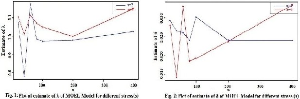
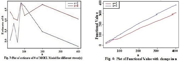
The proposed geometric method has several innovative and unique features. It deals with original parameter. Table 1 and 2 summarizes the results of the estimates for θ, λ & δ.

Based on the results of the simulation study, we observe

levels,”Journal of Statistical Planning and Inference, vol. 138, no. 3, pp. 78-786, 2008.

[9] Y. Lam, “Geometric Process and Replacement Problem, Acta

Mathematicae Applicatae Sinica,” vol. 4, no. 4, pp. 366-377, 1988.

[10] Y. Lam, “The geometric process and its application,”World

that estimates

ˆ , ˆ and ˆ

are quite well with relatively

Scientific Publishing Co. Pte.Ltd., Singapore, 2007.

small root mean squared and mean absolute error. This model work well for stress level s=4 and as the value of n increases the estimates become more stable. It should be noted that the bootstrap method demands a further computational complexity, in comparison with approximate confidence interval but it gives better results due to replication. Fig.1, Fig.2 & Fig.3 shows the variation of estimates for different sample values.From Fig. 4, we conclude that how with the increase in sample size the functional value also increases. Hence θ, λ & δ are not sensitive parameters.

Therefore, the test design obtained here is robust design and work well under the situation where no censoring occurs.

ACKNOWLEDGMENT

The first author wishes to thank Mr. Mohd Anjum,

[11] Y. Lam and S.K. Chan, “Statistical inference for geometric

processes with lognormal distribution”, Computational Statistics and Data Analysis, vol. 27, pp. 99-112, 1998.

[12] K. Zhou, Y.M. Shi and T.Y. Sun, “Reliability Analysis for

Accelerated Life-Test with Progressive Hybrid Censored Data Using Geometric Process, “Journal of Physical Sciences, vol. 16, pp. 133-143, 2012.

[13] A. N. Marshall and I.A. Olkin, “new method for adding a

parameter to a family of distributions with applications to the exponential and Weibull families,” Biometrica, vol. 84, pp. 641-

652, 1997.

[14] R.C. Gupta, M.E. Ghitany and Al-Mutairi. “Estimation of reliability from Marshall-Olkin Extended Lomax distribution”. Journal of Statistical Computation and Simulation, vol. 80, no. 8, pp.

937-947, 2010.

[15] A.K. Srivastava and V. Kumar. “Software Reliability Data Analysis with Marshall-Olkin Extended Weibull Model using MCMC Method for Non-Informative, Set of prior,” International

IJSER

Assistant Professor in Aligarh Muslim University for

valuable suggestions and help throughout my work which

substantially has improved this paper.

REFERENCES

[1] N. Ahmad, A. Islam, R. Kumar and R.K. Tuteja, “Optimal design of accelerated life test Plan under Periodic inspection and Type I censoring: The case of Rayleigh failure law,” South African Statistical journal, vol 28, pp. 27-35, 1994.

[2] Islam and N. Ahmad, “Optimal design of accelerated life test

plan for Weibull distribution under periodic inspection and Type

I censoring, “Microelectronics Reliability, vol. 34, no. 9, pp. 1459-

1468, 1994.

[3] N. Ahmad and A. Islam, “Optimal design of accelerated life test plan for Burr Type XII distribution under periodic inspection and Type I censoring,” Naval Research Logistics, vol. 43, pp. 1049-1077,

1996.

[4] N. Ahmad, A. Islam and A. Salam, “Analysis of optimal accelerated life test plan for periodic inspection: The case of exponential Weibull failure model,” International journal of Quality and Reliability Management, vol. 23, no. 8, pp. 1019-1046, 2006.

[5] N. Ahmad, “Designing Accelerated Life Test for Generalized

Exponential Distribution with Log linear Model,”International journal of Reliability and safety, vol. 4, no. 2/3, pp. 238-264, 2010.

[6] G. B. Yang, “Optimum constant stress accelerated life- test plan,

“IEEE Transactions on Reliability.” Vol.43 .no. 4, pp. 575-581, 1994.

[7] Z. Pan, N. Balakrishnan and Quan Sun, “Bivariate contant-stress accelerated degradation model and inference,” Communication in Statistics-Simulation and Computation, vol. 40, no. 2, pp. 247-257,

2011.

[8] A.J. Watkins and A.M. John, “On constant-stress accelerated life tests terminated by Type II censoring at one of the stress

Journal of Computer Applications, vol. 18, no. 4, pp. 31-39, 2011.

[16] G.S. Rao, “ A group acceptance sampling plans based on truncated life tests for marshall – olkin extended lomax distribution, “Electronic Journal Applied Statistical Analysis, vol. 3, no. 1, pp. 18-27, 2010.

[17] S. Shahab and A. Islam, “Analysis of accelerated life testing

using geometric process for frechet distribution,”International Journal of Innovative Research in Science, Engineering and Technology, vol. 2, no. 9, pp. 4987-4996, 2013.

IJSER © 2013 http://www.ijser.org