International Journal of Scientific & Engineering Research, Volume 4, Issue 7, July-2013 2292

ISSN 2229-5518

Comparison in Neural Network Method to Find Comparing Logistic Regression and Neural Network Model for Type 2 Diabetes Mellitus among Obesity

Sabri Ahmad, Tengku Nurhanis Tengku Adli, Aniza Abd Aziz, Jusoh Yacob

Abstract— Diabetes is a group of diseases marked by high levels of blood glucose, also called blood sugar, resulting from defects in insulin production, insulin action or both. Obesity are defined as a abnormal or excessive fat accumulation which may impair health. Obesity is the sixth most important risk factor that contributes to the burden of disease worldwide. Three objectives of building and find the best predictive model between Logistic Regression (LR) model and Neural Network (NN) model based on the value of predictive accuracy, sensitivity, specificity and the lowest error rate and to determine the factors that most contribute to risk among obesity. The primary data were obtained from diabetic clinic at Hospital Universiti Sains Malaysia (HUSM). Data were analyzed by using SPSS Clementine version 2.0 to constructed Logistic Regression (LR) and Neural Network (NN) model. At the end of the study, Prune method in NN is the best predictive model was strengthening by the result of lowest error rate and have quiet high sensitivity and specificity.

Index Terms— Type 2 Diabetes Mellitus, Obesity, Neural Network., Logistic Regression.

——————————  ——————————
error rate and to determine the most contributing factors

INTRODUCTION

Diabetes is a group of diseases marked by high levels of blood glucose, also called blood sugar, resulting from defects in insulin production, insulin action or both. Diabetes are divided into four types of diabetes such as type one diabetes, type two diabetes, gestational diabetes and pre-diabetes [1]. At present over 170 million people are living with diabetes across the globe. Around 3.2 mil- lion deaths every year are attributable to complications of diabetes; six deaths every minute. The top 10 countries, in numbers of sufferers are India, China, USA, Indonesia, Japan, Pakistan, Russia, Brazil, Italy and Bangladesh [1]. Obesity are defined as a abnormal or excessive fat accu- mulation which may impair health [2]. Obesity is the sixth most important risk factor that contributes to the burden of disease worldwide. The main adverse prob- lems are cardiovascular disease (CVD), type 2 diabetes mellitus (DM), and several cancers. The complications of overweight and obesity have achieved global problem during the past 10 years in contrast to malnutrition [3]. It is a common problem which affects not only affluent so- cieties but also developing countries. In terms of health impairment, besides being a disease in itself, obesity is a risk for many other diseases, mainly from the metabolic and cardiovascular area. Among these, type 2 diabetes, dyslipemia, hyperuricemia, arterial hypertension and cardiovascular disease are the most frequent [4]. The main objective of this study are to build and find the best predictive modeling such as Logistic Regression model (LR) and Neural Network model (NN) based on predictive accuracy, sensitivity, specificity and lowest

between independent variable such as age, gender, in- come, type of education, type of diabetic medication, family history diabetes mellitus, family history obesity, physical activity status, fiber intake/day and weight towards risk among obesity. The primary data were ob- tained from diabetic clinic at Hospital Universiti Sains Malaysia (HUSM). Data were analyzed by using SPSS Clementine version 2.0 to constructed Logistic Regression (LR) and Neural Network (NN) model. At the end of the study, Prune method in Neural network is the best predictive model was strengthening by the result of lowest error rate and has quiet high sensitivity and specificity.

1 MATERIAL AND METHODS

Data used in this study are primary data. This data was obtained from diabetic clinic at Hospital Universiti Sains Malaysia (HUSM). Factors affecting the risk of obesity problem listed in this study involving ten independent variables and one dependent variable. From 195 data, the data will split by training 70% and testing 30%. The vari- ables independent involved are age, gender, income, type of education, type of diabetic medication, family history diabetes mellitus, family history obesity, physical activity status, fiber intake/day and weight. Dependent variable (Y) takes the value 0 representing no risk to obesity and a value of 1 is the risk to obesity. The data
mining software SPSS Clementine version 12.0 was used for the purpose of building and find the best model. Three methods will be used for LR analysis which con- sists of methods Enter, Forwards and Backwards [5]. The

International Journal of Scientific & Engineering Research, Volume 4, Issue 7, July-2013 2293

ISSN 2229-5518

best LR model will be chosen as for comparison with
NN.
Enter are procedure for variable selection in which all variables in a block are entered in a single step. Forward Selection (Likelihood Ratio) are stepwise selection meth- od with entry testing based on the significance of the score statistic and removal testing based on the probabil- ity of a likelihood-ratio statistic based on the maximum partial likelihood estimates. Backward Elimination (Like- lihood Ratio) are backward stepwise selection removal testing is based on the probability of the likelihood-ratio statistic based on the maximum partial likelihood esti- mates [6].
Meanwhile there are 3 methods being used for NN mod- els which are Quick, RBFN and Prune. Quick method uses rules of thumb and characteristics of the data to choose an appropriate shape (topology) for the network. Radial Basis Function Network (RBFN) method using the same techniques to k-means clustering to some target data based on field values. Prune method starts with a large network and removes (Prunes) the weakest units in the hidden and input layers as training proceeds [7]. The best NN model will be chosen as for comparison with LR. The best method among LR and NN will be compared in order to identify the best predictive model. In order to determine which model is the best, the models will be evaluated based on Misclassification Rate (Error Rate), Predictive Accuracy (Classification Accuracy), Sensitivity and specificity [8]. It is used as a measure of the predic- tive performance of the predictive model. Misclassifica- tion rate is the percentage of misclassified observa- tions.

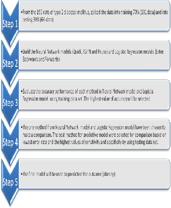
Figure 1: The summary of methodology for this study.

International Journal of Scientific & Engineering Research, Volume 4, Issue 7, July-2013 2294

ISSN 2229-5518

Table 1: The description of variables for this study.

Variable Role Measurement

Description

Level

Obesity Out Flag Body fat composition of patients
0: No Risk
1: At Risk
Age In Set Age of patients (Years)
1: 30-50
2: 51-70
3: 71-90
Gender In Flag Gender of patients
1: Male
2: Female
Income In Set Income / month (RM) of patients
1: 100-1000
2: 1001-2000
3:2001-3000
4: 3001-4000
5: 4001-5000
6: 5001-6000
7: 6001-7000
Type of education
(TypeOfEducation)
Type of diabetic medica- tion
(DrugDM)
Family history diabetes mellitus
(FhxDM)
Family history obesity
(FhxObesity)
Physical activity status
(Exercise)
Fiber intake/day
(FiberDiet)
In Set Type of education of patients
0: No education
1: Low education level
2: Intermediate education level
3: High
In Set Type of diabetic medication of patients
1: Oha
2: Insulin
3: Both
In Flag Family history diabetes mellitus of patients
1: Yes
2: No
In Flag Family history obesity of patients
1: Yes
2: No
In Flag Physical activity status of patients
1: Yes
2: No
In Set Fiber intake / day of patients
1: Once
2: Twice
3: Three times
4: Four times
5: Five and above
Weight In Set Weight of patients (kg)
1: 40-60
2: 61-80
3: 81-100

4: 101-120

International Journal of Scientific & Engineering Research, Volume 4, Issue 7, July-2013 2295

ISSN 2229-5518

3 RESULTS AND FINDINGS

From the fig. 2 below show the process flow diagram for LR

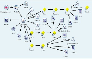
model and NN model using SPSS Clementine.
Figure 2: Process flow diagram for Logistic Regression model and
Neural Network model.
From the result for LR model, Forwards method for predictive model as it has the highest testing predictive accuracy which is 87.79%.
The estimated model is
other variables in the model (2) is constant.

Income

Logistic Regression coefficient estimates for income (1) is -
19.413 and the exponent is = 0.000. -19.413 value indicates if one unit increase in income category, limit ratio risk for no risk expected to decrease by -19.413 units. While the value of 0.000 shows that in the event of one unit increase in income, the type 2 diabetes is expected to risk for obesity by a factor of 0.000. In the case of the patient who has an income of RM100 to RM1000, the estimated is likely at risk 0.000 times.
Logistic Regression coefficient estimates for income (2) is -
18.495 and the exponent is = 0.000. -18.495 value indicates if one unit increase in income category, limit ratio risk for no risk expected to decrease by -18.495 units. While the value of 0.000 shows that in the event of one unit increase in income, the type 2 diabetes is expected to risk for obesity by a factor of 0.000. In the case of the patient who has an income of RM1001 to RM2000, the estimated is likely at risk 0.000 times.
Logistic Regression coefficient estimates for income (3) is -
17.894 and the exponent is = 0.000. -17.894 value indicates if one unit increase in income category, limit ratio risk for no risk expected to decrease by -17.894 units. While the value of 0.000 shows that in the event of one unit
Where:

P = 1

1 + e − z

(2)
(1)
increase in income, the type 2 diabetes is expected to risk for obesity by a factor of 0.000. In the case of the patient who has an income of RM2001 to RM3000, the estimated is likely at risk 0.000 times.
(
Logistic Regression coefficient estimates for income (4) is
0.774 and the exponent is = 2.168. 0.774 value indicates if one unit increase in income category, limit ratio risk for no risk expected to increase by 0.774 units. While the value of 2.168 shows that in the event of one unit increase in income, the type 2 diabetes is expected to risk for obesity by a factor of 2.168. In the case of the patient who has an income of RM3001 to RM4000, the estimated is
Detailed description of equation (2) is as follows:

Constant

Values for risk of obesity priority is 39.944. That is the ex- pectation value of the multinomial of risk to not risk when the values of variables in the model estimator (2) is empty.

Gender

Estimated Logistic Regression coefficients for gender (1) is -
1.958 and the exponent is = 0.141. -1.958 value indicates if one unit increase in gender category, log limit ratio risk for no risk expected to decrease by -1.958 units. While the value of 0.141 shows that in the event of one unit increase in gender, the type 2 diabetes is expected to risk for obesity by a factor of 0.141. In this case the male gender of patients, the estimated is likely at risk as 0.141 times when
likely at risk 2.168 times.
Logistic Regression coefficient estimates for income (5) is
0.308 and the exponent is = 1.360. 0.308 value indicates if one unit increase in income category, limit ratio risk for no risk expected to increase by 0.308 units. While the value of 1.360 shows that in the event of one unit increase in income, the type 2 diabetes is expected to risk for obesity by a factor of 1.360. In the case of the patient who has an income of RM4100 to RM5000, the estimated is likely at risk 1.360 times.
Logistic Regression coefficient estimates for income (6) is -
39.934 and the exponent is = 0.000. -39.934 value indicates if one unit increase in income category, limit ratio risk for no risk expected to decrease by -39.934 units. While

International Journal of Scientific & Engineering Research, Volume 4, Issue 7, July-2013 2296

ISSN 2229-5518

the value of 0.000 shows that in the event of one unit increase in income, the type 2 diabetes is expected to risk for obesity by a factor of 0.000. In the case of the patient who has an income of RM5100 to RM6000, the estimated is likely at risk 0.000 times.

Family history obesity

Logistic Regression coefficient estimates for family history obesity (1) is 2.070 and the exponent is = 7.924. 2.070 value indicates if one unit increase in family history obesity category, limit ratio risk for no risk expected to increase by
2.070 units. While the value of 7.924 shows that in the event of one unit increase in family history obesity, the type 2 diabetes is expected to risk for obesity by a factor of 7.924. In the case of the patient who has an family history obesity, the estimated is likely at risk 7.924 times.

Weight

Logistic Regression coefficient estimates for weight (1) is -
20.241 and the exponent is = 0.000. -20.241 value indicates if one unit increase in weight category, limit ratio risk for no risk expected to decrease by -20.241 units. While the value of 0.000 shows that in the event of one unit increase in weight, the type 2 diabetes is expected to risk for obesity by a factor of 0.000. In the case of the patient who has weight of 40 kg to 60 kg, the estimated is likely at risk
0.000 times.

Logistic Regression coefficient estimates for weight (2) is -
17.767 and the exponent is = 0.000. -17.767 value
indicates if one unit increase in weight category, limit ratio
risk for no risk expected to decrease by -17.767 units. While
the value of 0.000 shows that in the event of one unit
increase in weight, the type 2 diabetes is expected to risk for
obesity by a factor of 0.000. In the case of the patient who
has weight of 61 kg to 80 kg, the estimated is likely at risk
0.000 times.
Logistic Regression coefficient estimates for weight (3) is
15.676 and the exponent is = 6427195.205. 15.676 value indicates if one unit increase in weight category, limit ratio risk for no risk expected to increase by 15.676 units. While the value of 6427195.205 shows that in the event of one unit increase in weight, the type 2 diabetes is expected to risk for obesity by a factor of 6427195.205. In the case of the patient who has weight of 81 kg to 100 kg, the estimated is likely at risk 6427195.205 times.
From the result for NN model, Prune is the best predictive model as it has the highest testing predictive accuracy which is 90.08%.
Table 2 below show the full comparison between LR model (Forwards) and NN model (Prune) obviously shows that Prune has the lowest error rate which is 7.0% and have quiet high sensitivity and specificity.
Table 2: Comparison between Logistic Regression model and
Neural Network model.

For conclussion, the Prune method in NN model is the best model predictive to predict the risk in obesity because has successfully to fulfill the criteria to make a comparison and the important variable which is affected the obesity are weight and family history of obesity.

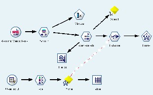
Figure 3: The Best Predictive Neural Network model (Prune) Finally, the NN model with Prune method has been choosen
to be the best model in predicted type 2 diabetes mellitus
towards obesity as shown at fig. 3.

4 CONCLUSION

For future study, some improvement can be made for a similar study that is by including more predictors’ variables in the models which are related to the obesity of type 2 diabetes mellitus. Furthermore, more number of observations should be included in the future research provided balance percent- age between at risk and no risk patients. Research to predict the performance of a type 2 diabetes mellitus that has a category of the dependent variables can be carried out using the other techniques that more advanced such as Support Vector Machine (SVM) or genetic algorithm. This study can be used to obtain information about the cause of the risk in obesity.

International Journal of Scientific & Engineering Research, Volume 4, Issue 7, July-2013 2297

ISSN 2229-5518

REFERENCES

[1] Misnadiarly. (2006). Diabetes Melitus Gangren, Ulcer, Infeksi, Mengenali gejala, Menanggulangi, dan Mencegah komplikasi. Jakarta: Pustaka Obor Populer.

[2] WHO, W. H. O. (2006). Obesity and overweight. [Online] [Accessed

11/3/2010, 2010], Available from World Wide

Web:http://www.who.int/mediacentre/factsheets/fs311/en/.

[3] Haslam, D. W. & James, W. P. (2005). Obesity.Lancet, 366 (9492), 1197-

209.

[4] Formiguera, X. & Canton, A. (2004). Obesity: epidedemiology and clinical aspects. Best Pract Res Clin Gastroenterol, 18 (6), 1125-46.

[5] Levin, R.I. & Rubin, D.S. (1994). Statistics for Management. 6th ed.

Englewood Cliffs, N.J.: Prentice Hall. pp. 646-693

[6] Hosmer DW, Lemeshow S. Applied Logisric Regression. New York, John Wiley & Sons;1989. Guertiete MRJ, Decsky AS. Neural networks:What are they? Ann Intern Med 1991;115: 906-907

[7] White H. Learning in artificial neural networks: A statistical perspectives. Neural Comput 1989; 1: 425-464

[8]Dr. Masoud Y., Neural Network Algorithms, SPSSN

clementime12.0;2010:1-7