International Journal of Scientific & Engineering Research, Volume 6, Issue 1, January-2015

ISSN 2229-5518

1311

Comparing Decision Tree Classifier Models for

Deriving Optimized Rules

Anita Chaware, Dr.U.A. Lanjewar

Abstract— This paper evaluates the Different Decision tree classifiers performance on the basis of statistical indices like sensitivity and specificity and the generated confusion matrics. Our research is to find the best classifiers which generate the tree. This will help us to obtain the optimiesd rules from the tree. This research uses 5 different classifiers namely, Ramdom tree, NBTree, Simple Cart , ID3, J48. WEKA software, a open source collection of machine learning tools to generate the Classifiers tree model. The accuracy performance measures based on the statistical indices, like the confusion matric is used to comapare the models performance. Looking at the skewed type of database, the research further included the performance measures AUC(area under curve) for each generated model and finally compares all the AUC to get the best performer. The experimental results shows that the NBtree followed by J48 can be used as good classifiers for prediction in the skewed dataset or where the dataset in which cost of misclassification is much higher.

Index Terms—Decision tree classifier, Sensitivity and Specificity analysis, AUC, rules genartion,

——————————  ——————————

1. INTRODUCTION

Any data needs to be statistically analysed to get information. With enormous volumes of data, Analysers are finding differ- ent methods and techniques to analyze the data and dig the important information hidden in this data mines. Main rea- sons to use data mining are the huge data and less infor- mation. One need to to extract the information, analyze and interpret it to get very valuable knowledge which they could not otherwise find. The hidden patterns which data mining is able to handle are classification, forecasting, Rule extraction, Sequence detection, clustering,etc. Classification is to classify an object into one or more class or category, based on its other characteristics. For examples, in education, teachers and in- structors are all the time classifying their students for their knowledge, motivation, and behaviour. Assessing exam an- swers is also a classification task, where a mark is determined according to certain evaluation criteria[1,2]. Automatic classi- fication is an inevitable part of any intelligent system used for predictions. Before the system can predict any action like stu- dents selecting subject , Acedemic factors like marks, learning material, or advice, it should first classify the students historic data. For this purpose, we need a classifier – a model, which predicts the class value from other explanatory attributes. Such predictions are equally useful in the teaching learning process of the Acedemics. [3].
Classifiers can be designed manually, based on expert’s
knowledge, but nowadays it is more common to learn them
from real data. The basic idea is the following: First, we have
to choose the classification method, like Decision Trees, Bayes-
ian Networks, or Neural Networks. Second, we need a sample
of data, where all class values are known. The data is divided
into two parts, a training set and a test set. The training set is
given to a learning algorithm, which derives a classifier. Then
the classifier is tested with the test set, where all class values
are hidden. If the classifier classifies most cases in the test set
correctly, we can assume that it works accurately also on the future data. On the other hand, if the classifier makes too many errors (misclassifications) in the test data, we can as- sume that it was a wrong model. A better model can be
searched after modifying the data, changing the settings of the learning algorithm, or by using another classification method. The basic forms of classifiers are called discriminative, be- cause they determine just one class value for each row of data. If M is a classifier (model), C = {c } the set of class values, and t a row of data, then the predicted class is M(t) = c1, ..., cli for just one i.
An alternative is a probabilistic classifier, which defines the probability of classes for all classified rows. Now M(t) = [P(C = c1 |t), ..., P(C = c |t)], where P(C = ci |t) is the probability that t belongs to class c.[4]
Probabilistic classification contains more information, which
can be useful in some applications. Like in case where one
should predict the student’s performance in a course, before
the course has finished. The data often contains many incon-
sistent rows, where all other attribute values are the same, but
the class values are different. Therefore, the class values can-
not be determined accurately, and it is more informative for
the course instructors to know how likely the student will pass
the course. It can also be pedagogically wiser to tell the stu-
dent that she or he has 48% probability to pass the course than
to inform that she or he is going to fail.

1.1 Types of classifeiers

Major types of classifiers are decision trees, Bayesian classifiers, Neural Networks, Nearest Neighclassifiers, Sup- port Vector Machines, and Linear Regression[5]. The approach compared for their suitability to classify typical educational data. The study here is limited to the different decision trees as they gererates the rules in form of the tree. Decision tree classi- fier is one of the possible approaches to multistage decision in form of rules which can be further used in application of fuzzy rule. The basic idea involved in any multistage approach is to break up a complex decision into a union of several simpler decisions, hoping the final solution obtained this way would resemble the intended desired solution.[7]

IJSER © 20 1

http://www.ijser.org

International Journal of Scientific & Engineering Research, Volume 6, Issue 1, January-2015

ISSN 2229-5518

1312

1.2 Evaluation measures of Classification

The performance of each classification model is evaluated on the basis of accuracy which is is further calculated using the Confusion Matric.
Confusion matric is a n dimension table showing the counts of correctly and not correctly classified counts of the test re- cords, predicted by the Classifier Model.[9] Ecah cell Cij de- notes the count of the records from class i predicted to be the class j , by the model.
The columnwise value are predicted and row wise are ac- cual for each Cij, i=j the values are correctly/ truly classified values and are shown as tpA rest are wrongly predicted count shown by eAB. The total of row or column gives the total num- ber of data records. The sensitivity, specificity and accuracy values are obtained from this tpA and eAB. The formulas are explained below in eq 1, eq 2, and eq 3 respectively
Predicted class
Confusion matrics A B C
SensitivityA = tpA/(tpA+eAB+eAC) (1) SpecificityA = tnA/(tnA+eBA+eCA), (2)
where tnA = tpB + eBC + eCB + tpC
tpA+ tpB+ tpC
Accuracy = -------------------------------------------------- (3)
tpA+eAB+eAC+eBA+tpB + eBC + eCA +eCB +tpC

1.3 AUC (area under the ROC curve)

A common method is to calculate the area under the ROC curve, abbreviated AUC [9]. ROC graphs are two-dimensional graphs in which tp rate is plotted on the Y axis and fp rate is plotted on the X axis. An ROC graph depicts relative tradeoffs between benefits (true positives) and costs (false positives). Since the AUC is a portion of the area of the unit square, its value will always be between 0 and 1.0. However, because random guessing produces the diagonal line between (0, 0)
and (1, 1), which has an area of 0.5, no realistic classifier
should have an AUC less than 0.5.
Several points in ROC space are important to note. The lower left point (0, 0) represents the strategy of never issuing a posi- tive classification; such a classifier commits no false positive errors but also gains no true positives. The opposite strategy, of unconditionally issuing positive classifications, is repre- sented by the upper right point (1, 1). The point nearing to (0,
1) represents perfect classification(optimistic sequence). i.e. one point in ROC space is better than another if it is to the northwest (tp rate is higher, fp rate is lower, or both) of the first. The point very far away from (0,1) are pessimistic se- quence and make the model a poor model. Between optimistic and pessimistic the expected sequences should fall more to-
ward the northwast to make the classifier model perform bet- ter. The curves are explain in fig.1.

Fig.1. ROC curves showing the optimistic, pessimistic and expected s e- quences of the classifier model.

A perfect classifier has AUC=1 and produces error-free deci- sions for all instances. A perfectly worthless classifier has AUC=0.5 and consists of the locus of points on the diagonal line xy = from (0,0) to (1,1)[10]. It represents a random model that is no better at assigning classes than flipping a fair two- sided coin.

1.4 Overview

The rest of the chapter is organized as follows: In Section 2, we defines and discuss the different decision tree and their accu- racy calculation procedure. In Section 3, we presents the ex- perimental procedure and analyze their suitability to the edu- cational domain. Section 4, presents the results and compare them by drawing the conclusions in section 5.

2. DECISION TREE CLASSIFIER

The decision tree classifier uses a layered or hierarchical ap- proach to classification. It is a simple structure that uses greedy approach like divide and conquer technique to break down a complex decision making process into a collection of simpler decisions, thereby providing an easily interpretable solution [11], [12]. The decision tree thus generated is trans-
parent and we can follow a tree structure easily to see how the
decisions are made [12]. It is a predictive modeling technique
used in classification, clustering and prediction tasks. In deci-
sion tree the root and each internal node are labeled
Each leaf node represents a prediction of a solution to the
problem under consideration.
Given some training data T, the ideal solution would test all possible sequences of actions on the attributes of T in order to find the sequence resulting in the minimum number of mis- classifications.
The main objectives of decision tree classifiers are: 1) to classi- fy correctly as much of the training sample as possible; 2) gen- eralize beyond the training sample so that unseen samples could be classified with as high of an accuracy as possible; 3) be easy to update as more training sample becomes available;
4) to have as simple a structure as possible.

IJSER © 20 1

http://www.ijser.org

International Journal of Scientific & Engineering Research, Volume 6, Issue 1, January-2015

ISSN 2229-5518

I

1313

In Decision tree classification, the most popular measure of performance is the misclassification rate, which is simply the percentage of cases misclassified by the model. We have used the same misclassification or error rate for our comparison of the five decision tree classifiers.

2.1 Types of Decision Tree Classifiers

The different types of decision trees are Ramdom tree, RandomForest, NBTree, SimpleCart, ID3, C4.5 its veriant J48,CART, SPLINT,etc..

2.2 Data Discribtion

The dataset used in this research work is of acedemic data of students. It has 150 instances with 6 attributes out of which none have one or more missing values. The data set contains good mix of attributescontinuous, nominal with small num- bers of values, and nominal with larger numbers ovalues. For the purposes of training and testing, only 75% of the overall data is used fotraining and the rest is used for testing the accu- racy of the classification of the selecteclassification methods.

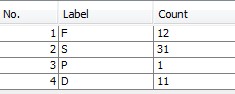
Fig.2 Table generated by weka for counting the diffent classes called as labels and their counts

3. MATHODOLOGY

In this section, we have applied the different decision tree ex- plained in the Section 2 on the acedemic data aiming to inves- tigate their effectiveness in generating the optimized rules. The confusion matrix in each case is given which is obtained from WEKA , a open source Machine Learning tool devolped by the Weiktando University research students. It has a free collection of nearly all ML algorithms. The Sensitivity and specificity and the accuracy of the each algorithm is given along with the confusion matrix. These parameters are calcu- lated using the formula given in section 1.2.
In order to improve performance estimate of the algorithms used in this paper, the datasets described in Section 2.2 were divided with the 10-fold stratified cross-validation methodol- ogy. Accordingly, each dataset was divided into 10 subsets of approximately equal size, with 50% of presence data and 50% of absence data.
For each ML technique, the examples from 9 folds are used to
train a classifier, which is further evaluated in the remaining
fold. This process is repeated 10 times, using at each cycle a different fold for test. The performance of each classifier is given by the average of the performances observed in the test folds. The AUC (Area Under the ROC Curve) was used to evaluate the classifiers effectiveness in the classification of preence/absence data as explained in section 2.3.

4. EXPERIMENT

The whole experiment was done in weka software, which needs the data files in special format like .csv, .arff(default format) and many more. As our data was in excel format we converted the excel file into the csv format to work with WE- KA. The following trees Ramdom tree, NBTree, SimpleCart, ID3, J48 were selected to evaluate their performance based on the model statistics and AUC.

4.1 RandomTree

RandomTree are predictors. The tree votes for its preferred
class and the most voted class gives the final prediction.
Let T be a training dataset with n data items and where each
item has m attributes. For each tree, a new training dataset T1
is built by sampling T at random with replacement (bootstrap
sampling)[13]
To determine a node split in the tree, a subset m m of the
atributes is chosen at random. The best split of these selected
attributes is then used. The trees are grown in order to classify
all data items from T0 correctly and there is no pruning. The
value m can be chosen based on an out-of-bag error rate esti- mate. RFs have been successful in a wide range of applications and are fast to train. also showed that RFs do not overfit, de- spite the number of trees employed in the combination.
The confusion matrix generated by the weka software for the
RandomTree classifer model is given in Fig.3.
RandomTree a b c sensitivity a=D 17 9 0 0.65
b=F 9 20 1 0.30 c=S 0 1 0 0.00
Specificity 0.71 0.63 0.98
Accuracy 0.65

Fig.3. Confusion matrics and the accuracy measure of the Model.

4.2 NBTrees

A decision tree is built with univariate splits at each node But with Naïve Bayes classiers at the leaves. The final classifier resembles to Utogoff’s Perceptron trees . But the induction process is very different andgeared toward larger datasets. The decision tree segments the data a task that is consider an essential part of the data mining process in large databases. Each segment of the data represented by a leaf is described through a Naïve Bayes classier[14].

IJSER © 20 1

http://www.ijser.org

International Journal of Scientific & Engineering Research, Volume 6, Issue 1, January-2015

ISSN 2229-5518

1314

Fig.4. Confusion matrics and the accuracy measure of the Model gen- erated by NBTree

4.3 SimpleCart

Builds multivariate decision (binary) trees known as CART commonly n SimpleCart in WEKA. The CART or Classifica- tion & Regression Trees methodology was introduced in 1984 by Leo Breiman, Jerome Friedman, Richard Olshen and Charles Stone as an umbrella term to refer to the following types of decision tree:
Classification Trees: where the target variable is categori- cal and the tree is used to identify the "class" within which a target variable would likely fall into
Regression Trees : where the target variable is continuous and tree is used to predict its value.

Fig.5. Confusion matrics and the accuracy measure of the Model gen- erated by SimpleCart

4.4 ID3

ID3 is a simple decision learning algorithm developed by J. Ross Quinlan in 1986. ID3 constructs decision tree by employing a top-down, greedy search through the given sets of training data to test each attribute at every node. It uses statistical property call information gain to select which attribute to test at each node in the tree. Information gain measures how well a given attribute separates the training examples according to their target classification.

4.5 J48

J48 is an open source Java implementation of the C4.5 algo- rithm in the Weka data mining tool. C4.5 is a program that creates a decision tree based on a set of labeled input data. This algorithm was developed by Ross Quinlan. The decision trees generated by C4.5 can be used for classification, and for this reason, C4.5 is often referred to as a statistical classifier (”C4.5 (J48)”, Wikipedia).
J48 tree a b C sensitivity a=D 22 4 0 0.85
b=F 6 21 1 0.21 c=S 0 1 0 0.00
Specificity 0.79 0.81 0.98
Accuracy 0.78

Fig.7. Confusion matrics and the accuracy measure of the Model gen- erated by J48 a Weka verient of c4.5

5. RESULTS COMPARISION ABD ANALYSIS

5.1 Results from Confusion matrics

After building the models using the training data, and predict- ing the Classes of acedemic data category for each given input in the testing data, we obtain the confusion matrix for each model, and then compute the sensitivity and specificity as de- scribed in Section 3.1. Table 6 shows the sensitivity and speci- ficity for each of the four models’ categories, namely D,F,S…

FIG. 8. TABLE SHOWING SENSITIVITY , SPECIFICITY AND ACCURACY

Fig.6. Confusion matrics and the accuracy measure of the Model gen- erated by ID3

From Table in Fig.8., it seems that the J48 Does a better job in
prediction as compared to the SimpleCart which is much clos-
er to it followed by ID3, NBTree, RandomTree in order of their
accuracy thus calculated from equation 3 0f section 3.

IJSER © 20 1

http://www.ijser.org

International Journal of Scientific & Engineering Research, Volume 6, Issue 1, January-2015

ISSN 2229-5518

1315

The Sensitivity and Specificity thus optained from the confu- sion matric can not be totally belived as appropriate cost sensi- tive analysis as we can see from the above comaprision that for the class S the sensitivity is 0 everywhere. This is because the data which we are considering for this research is having many instances labled as D , few as F and very less as S. the classifiers blindly tell everything as Either D or F as the S class instsances are very few. This type of classifiers are assumed as bad classifiers but their accuracy rate ic correct as atleast they are correctly identifying the Class D,S and F instance labels. But they are not identifying the Class P instance labels.the ac- tual instances labels are shown in Fig.1. So these measures of sensitivity and specificity are not reflecting the appropriate accuracy of the classifiers. i.e. a classifier may be preferred to another based on the fact that it has better prediction accuracy than its competitor[15]. Without additional information de- scribing the cost of a misclassification, accuracy alone as a se- lection criterion may not be a sufficiently robust measure when the distribution of classes is greatly skewed or the costs of different types of errors may be signifi- cantly dif erent.

5.2 Results from AOC

Model RandomTree

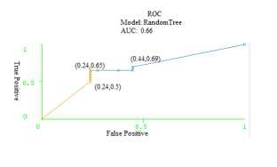
Fig.9. ROC showing the AUC for the Model Random tree

Model SimpleCart

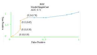
Fig.10.ROC showing the AUC for the Model SimpleCart
Model NBTree

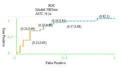
Fig.11. ROC showing the AUC for Model NBTree
Model ID3

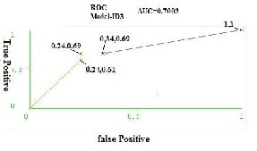
Fig.12. ROC showing the AUC for the Model ID3

Model J48:

Fig.13.ROC showing AUC for the Model J48 .

IJSER © 20 1

http://www.ijser.org

International Journal of Scientific & Engineering Research, Volume 6, Issue 1, January-2015

ISSN 2229-5518

1316

5.3 Comparision and Analysis of AUC

The WEKA tool generated the Classifiers model and along with it it gives all the statistical information. It also gives the AUC curve values when left clicked on the selected model . All the models AUC values were noted down and compared with the each other. The model NBTree gives more promising results with respect to AUC value. The comparative statement is given in fig.14.

Fig.14 Comparative statement of AUC values for all models.

6. CONCLUSION

In this paper, a research effort were done to developed several Classification models for Students acedemic data. Specifically, we used five popular data mining – machine learning algo- rithms namely, RndomTree, SimpleCart, NBTree, ID3, J48 a WEKA verient for C4.5. the database used was a simple csv format file having students Acedemic data. In order to measure the unbiased accuracy of the five classifiers model,we used a 10- fold cross-validation procedure. That is, WEKA divides the data- set into 10 mutually exclusive partitions (a.k.a. folds) using a stratified sampling technique. Then, 9 of 10 folds are used for training and the 10th for the testing. This process is repeated for

10 times so that each and every data point would be used as part of the training and testing datasets. The accuracy measure for the model is calculated by averaging the 10 models performance numbers. In this paper, We repeated this process for each of the Five classifiers. This provided us with a less biased prediction performance measures to compare the tree models. The aggre- gated results indicated that the J48 is more promising with re- spect to the sensitivity and specificity i.e. accuracy measures.

In detail when accuracy is the factor than RandomTree gives 65%

of accuracy, NBTree gives 67% of accuracy, Simple cart gives

73% of accuracy, ID3 gives 69% and J48 gives the highest i.e.

78% of accuracy while classifying the classess.

Where as with respect to the ROC , the AUC values for all there trees are very different. RandomTree gives 66% of accuracy, NBTree gives the highest i.e. 79% of accuracy, Simple cart gives

72% of accuracy, ID3 gives 70% and J48 gives. 78% of accuracy while classifying the classess. This also shows that dataset with various size matters a lot in the performance calculation of the classifiers. i.e. same classifiers behaves differently with different datasets[16]. Since the students data was skewed type of the clas- sifier has misclassified the values and hence the accuracy values are different than the AUC vlues for the same dataset and same classifiers. NBTree shows remarkable performance with AUC wheras, is of no use to us when the measures are statistical. J48 show a constant pattern of performance in both the cases. Fig. 15 gives the comparitative statements of the Accuacy measures and the AUC measures of each classifer models.

Fig.15 comparative statement of performance factors like accu- racy and AUC for the different Clssifiers.

REFERENCES

[1] Ali Buldua, Kerem Ucgin, “Data mining application on students’ da- ta.”, Procedia Social and Behavioral Sciences , 5251–5259, 2010

[2] Baradwaj, Brijesh Kumar, and Saurabh Pal, “Mining Educational Data to Analyze Students' Performance”, ArXiv , 1201-3417, 2012.

[3] Romero, C., S. Ventura, P.G. P.G. Espejo, and C. Hervas, “ Data mining algorithms to classify students.”, Proceedingsof the 1st international conference on educational data mining, 8–17, 2008.

[4] Hamalainen W., and M. Vinni. “Comparison of machine learning

methods for intelligent tutoring systems.”, In Proceedings of the 8th international conference on intelligent tutoring systems, vol. 4053 of Lecture Notes Computer Science, 525–534. Springer-Verlag, 2006.

[5] R.P.W. Duin, “A Note on Comparing Classifiers”, Pattern Recognition

Letters 17 ,1996

[6] Kumar, Varun, and Anupama Chadha, “ Mining Association Rules in Student’s Assessment Data.”, International Journal of Computer Sci- ence Issues 9,vol.5, 211-216, 2012.

[7] G. R. Dattatreya and L. N. Kanal, " Decision trees in pattern recogni- tion," In Progress in Pattern Recognition 2, Elsevier Science Publisher B.V., 189-239 1985.

[8] A. V. Kulkarni and L. N. Kanal, "An optimization approach to hiera r- chical classifier design," Proc. 3rd Int. Joint Conf. on Pattern Recogni- tion, San Diego, CA, 1976.

[9] Tom Fawcett, “An introduction to ROC analysis”, Pattern Recognition

Letters 27,861–874, 2006.

[10] Bradley, A.P., “The use of the area under the ROC curve in the evalua-

tion of machine learning algorithms”, Pattern Recogn. 30 (7), 1145–

1159,1987.

[11] Quinlan, J. R., “Introduction of decision trees”, Machine Learning, 1, pp

81-106, 1986

[12] Quinlan, J. R. ,“Simplifying Decision Trees”, The MIT Press, 1986.

[13] L. Breiman. Random forests. Machine Learning, 45(1): 5–32, 18, 2001 [14] R. Kohavi, “Scaling Up the Accuracy of Naive-Bayes Classifiers: a De-

cision-Tree Hybrid “, Proceedings of the Second International Confer-

ence on Knowledge Discovery and Data Mining, 1996

[15] Demsar, J. , “ Statistical comparisons of classifiers over multiple da-

tasets”, Journal of Machine Learning Research, 7, 1–30.2006.

[16] Adams, N.M., and D. J. Hand , “ Comparing Classifiers When the Mis- allocation Costs are Uncertain”, . Pattern Recognition, Vol. 32, No. 7, pp. 1139-1147,1999.

[17] B.K. Bharadwaj and S. Pal. “Mining Educational Data to Analyze Stu-

dents Performance”, International Journal of AdvanceComputer Sci-

ence and Applications (IJACSA), Vol. 2, No. 6, pp.63-69, 2011.

[18] Dorina Kabakchieva, “Student Performance Prediction by using Data

Mining Classification Algorithms”,.I JC S MR , issue 4 November , ISSN 2278-733X .2011

[19] Zlatkok J.Kovacic “predicting Success by Mining Enrolment data”,

Research in Higher Education Journal.

[20] Weka 3- Data Mining with open source machine learning software

available from :- http://www.cs.waikato. ac.nz/ml/ weka

IJSER © 20 1

http://www.ijser.org