International Journal of Scientific & Engineering Research, Volume 4, Issue 12, December-2013 2038

ISSN 2229-5518

Combined Estimators as Alternative to Feasible

Generalized Least Square Estimators

Kayode Ayinde

Department of Statistics

Ladoke Akintola University of Technology, P.M.B.4000, Ogbomoso, Oyo State, Nigeria

Email: bayoayinde@yahoo.com/ kayinde@lautech.edu.ng .

Abstract: Although the performances of the Feasible Generalized Least Square (FGLS) estimators developed to tackle violation of homoscedacity variance in linear regression model are asymptotically equivalent, their performances in small sample sizes still pose research challenges. In this paper, two FGLS estimators, CORC and ML estimators were combined with the estimator based on Principal Component (PC) Analysis and the Mean Square Error (MSE) sampling property criterion was used to examine and compare their performances through Monte Carlo Simulation study with both normally and uniformly distributed variables as regressors. The estimators were ranked at each level of autocorrelations and sample sizes and the sum of their

ranks as well as the number of times each estimator has the minimum MSE was obtained. Results show that out of all the combined estimators pro- posed, the CORCPC123 and MLPC123 generally performed better than or compete with their separate counterpart. They are asymptotically equivalent. At small sample size (n=10), the proposed estimator CORCPC123 is conspicuously more efficient than CORC; and with uniformly distributed regressors, the CORCPC12 is best at high level of negative autocorrelation. At low level of autocorrelation, the OLS estimator is generally most efficient while the PC12 is best with uniformly distributed regressors when the sample size is small (n=10).

Keywords: OLS Estimator, FGLS Estimators, Combined Estimators, Sampling Properties, Linear Regression Model.

IJSER

1 INTRODUCTION

——————————  ——————————

The Generalized Linear Model resulting from violation of the assumption of homoscedastic variance of the classical linear

and

σ 2 = σ 2 u =

σ 2 ε

, and the inverse of Ω is

regression model and loss of efficiency of the OLS estimator being used to estimate its parameters led to the development of the Generalized Least Square (GLS) estimator by Aitken [1].

(1 − ρ 2 )

 1 − ρ

0 3 0 0 

This GLS estimator βgiven as β=(X1Ω1X )-1 X1Ω1Y is efficient

among the class of linear unbiased estimators of β with vari- ance – covariance matrix of β given as V(β) = σ2(X1Ω1X)-1,

− ρ

 0



1 + ρ 2

− ρ

− ρ 3 0 

1 + ρ 2 3 0 0 



−1 1  . .

. 3 . . 

where Ω is assumed to be known. The GLS estimator de-

scribed requires Ω, and in particular ρ to be known before the

Ω =

(1 − ρ 2 )  . .



 . .

. 3 . . 



. 3 . . 

parameters can be estimated. Thus, in linear model with auto-

correlated error terms having AR (1):

 0 0



0 3 1 + ρ 2

− ρ 



1 −1

−1 1 −1

 0 0

0 3 − ρ

1 

(GLS )

2 1

X Ω Y

−1 −1

(1)

Now with a suitable (n-1) x n matrix transformation P* defined

V (βˆ

GLS ) ) = σ

( X Ω X )

(2) 0



where

 1 ρ



ρ 2 2

ρ n − 2

n − 3

ρ n −1 

n − 2 

P* =  .

 .



0



. . 3 . 

. . 3 . . 



 ρ 1

ρ 3 ρ ρ 

 . .



. 3 . . 



 .ρ 2 ρ



1 3 ρ n − 4

ρ n − 3 



 0 0

0 3 − ρ

1 ( n −1) + n

E (UU ′) = σ 2Ω = σ 2  .

. . 3 .

.  Multiplying then shows that

P *′ P *

gives an n x n matrix

 . .



 . .

. 3 .

.  which, apart from a proportional constant, is identical with

.  Ω −1 except for the first elements in the leading diagonal,

 ρ n − 2



ρ n − 3

ρ n − 4 1 ρ 



which is

ρ 2 rather than unity. With another n x n transfor-

 ρ n −1

ρ n − 2

ρ n − 3 3 ρ

1 

mation matrix P obtained from P* by adding a new row with

International Journal of Scientific & Engineering Research, Volume 4, Issue 12, December-2013 2039

ISSN 2229-5518

1 − ρ 2

in the first position and zero elsewhere, that is

problem. Just like the Principal Component does its estima- tion using the OLS estimator by regressesing the extracted components (PCs) on the standardized dependent variable, the combined estimators use the FGLS estimators,

(1 − ρ ) 2



 − ρ

 0



P =  .



 .

0 0 0 0



1 0 3 0 0

− ρ 1 0 0



. . 3 . . 

. . 3 . 

Cochrane and Orcutt (CORC) estimator [5] and the Maxi- mum Likelihood (ML) estimator [10], by regressesing the extracted components (PCs) on the standardized depend- ent variable. Unlike the OLS estimator which results back into the OLS estimator when all the PCs are used [15, 16]; advantageously, since the FGLS estimators require an iter-

Multiplying shows that P′P = (1 − ρ 2 )Ω −1 . The difference between P* and P lies only in the treatment of the first sample observation. However, when n is large, the difference is negli- gible, but in small sample, the difference can be major [2, 3]. The GLS estimation in (1) and (2) requires that Ω or more pre-

ble estimators when all the possible PCs are used for the estimation. Consequently, the parameters of (3) are esti- mated by the following eleven (11) estimators: OLS, PC1, PC12, CORC, CORCPC1, CORCPC12, CORCPC123, ML, MLPC1, MLPC12 and MLPC123 estimators.

For the Monte-Carlo simulation study, two types of re-

cisely ρ to be known but this is not often the case as ρ (or

hence Ω) is always estimated via the transformation matrix P*

gessors namely,

X i ~ N (0,1)

and

X i ~ U (0,1) were

and P and the use of the OLS estimator to get a consistent estimator ρˆ and have a Feasible Generalized Least Squares

Estimator (FGLS).There are several ways of consistently esti- mating ρ using either the P* or P transformation matrix [4]. Several developed FGLS estimators include the estimator provided by Cochrane and Orcutt [5], Paris and Winstern [6],

used.The parameters of equation (3) were specified and

fixed asβ0 = 4, β1 = 2.5, β2 = 1.8 and β3 = 0.6. Further- more, the experiment was replicated in 1000 times (R

=1000) under four (4) levels of sample sizes (n =10, 20, 30 and 100) and twenty – one levels of autocorrelation

( ρ = −0.99,−0.9,−0.8,...,0.8,0.9,0.99. ). The estimators

IJSER

Hildreth and Lu [7], Durbin [8], Theil [9], the Beach and Macki-

non [10] and Thornton [11]. Among others, the Maximum Like- lihood and Maximum Likelihood Grid proposed by Beach and

were evaluated and compared using the Mean Square Er-

ror Criterion since the separate estimator especially CORC

has been reported biased in small sample size Rao and

Mackinon [10] impose stationary by constraining the serial

correlation coefficient to be between -1 and 1 and keep the

Griliches [12]. Mathematically, for any estimator

βi of

βi i

first observation for estimation while that of Cochrane and Orcutt and Hildreth and Lu drop the first observation. Rao and Griliches [12] did one of the earliest Monte-Carlo investiga-

= 0, 1, 2, 3 the Mean Square Error (MSE) property of the estimator is defined as:

^ R  ^ 

tions on the small sample properties of several two-stage re-

MSE(β

) = 1 ∑  β

− β 

(4)

gression methods in the context of autocorrelated error terms. His findings, among other things, pointed out the inefficiency of these estimators especially the CORC estimator when the sample size is small. The Principal Component Analysis sug- gested by Massy [13] is being used for data reduction and also as a method of estimation of model parameters in the pres- ence of multicolliearity [14, 15, 16].

In view of the fact that the feasible generalized least square estimators, especially the CORC estimator, is inefficient in small sample size, this paper attempts to improve the efficien- cy of these estimators by combining them with the estimator based on Principal Component Analysis and examines the mean Square error sampling property of the resulting estima- tors.

2 MATERIALS AND METHODS

Consider the linear regression model of the form:

i R  ij i 

j =1  

For all these estimators, a computer program was written using Time Series Processor [17] software to evaluate Mean Square Error of the estimators on the parameters of the model. The estimators were ranked at each particular level of autocorrelations, sample sizes and the model pa- rameters and the sum of the ranks as well as the number of times each estimator has minimum MSE was used as a basis to identify the best estimator. An estimator is best at each particular level of autocorrelation and sample size if the sum of ranks is minimum and / or has highest number of minimum MSE.

3 RESULTS AND DISCUSSION

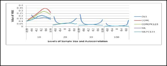
The results of the performances of five (5) generally com- peting estimators are graphically represented for the nor-

Yt = β0 + β1 X1t + β2 X 2t + β3 X 3t + Ut

(3)

mally distributed regressors. These are OLS, CORC, CORCPC123, ML and ML PC123. Figures 1A-1D and, 2A

Where Ut = ρUt −1 + ε t , ε t

~ N (0, σ

) ,t = 1, 2, 3,...n.

AND 2Bshow the graphical representation of the perfor- mances of the estimators with normally distributed re-

The technique adopted for the development of the com-

bined estimator is very much similar to that of the Principal

Component Estimator when used to solve multicollinearity

gessorson

β1 ,

β2 and

β3 respectively. The performances

International Journal of Scientific & Engineering Research, Volume 4, Issue 12, December-2013 2040

ISSN 2229-5518

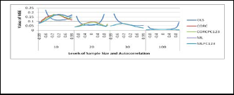
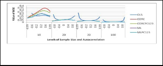
of the estimators with uniform regressors follow the same pattern even though the estimators perform much better with normal regressors (see Figure 1 and 2). From the fig- ures, the OLS estimator is best at low level of autocorrela- tion while the other ones only compete especially with in- creased sample size. This has also been noted and report- ed by many authors including Rao and Griliches [12] and Ayinde and Olaomi [18]. Furthermore, it can be easily seen that the estimators differ very significantly at small sample size, n=10, and that of CORC and ML with their proposed counterparts perform equivalently as the sample size in- creases. When the sample size is small (n=10), the alterna- tive combined estimator CORCPC123 is more efficient than the CORC while the MLPC123 is slightly more efficient es- pecially when the autocorrelation level is positive. The per- formances of the estimators are also affected by different type of regressors.

Error at each parameter level, summing their ranks over the model parameters and obtaining the number of times each estimator has the minimum MSE, at various levels of auto- correlation and sample size are presented in Table 2A and

2B. and 3.These estimators are OLS, PC1, CORC, ML, CORCPC12, CORCPC123, MLPC12 and MLPC123.

Table 1A: Summary Table of the total ranks of the estima- tors at various levels of autocorrelation and sample size.

Normal Regressors

Autocorrelation value

1
0

Fig. 1: Graphical Representation of the Mean Square Error of

β of some of the estimators with normally distributed regressors.

2
0

β2 of some of the estimators with normally distributed regressors.

3
0

Fig. 3: Graphical Representation of the Mean Square Error of

β3 of some of th estimators with normally distributed regressors.

0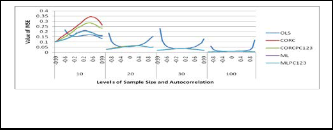

0

Fig. 4: Graphical Representation of the Mean Square Error of

β of some of th estimators with uniformlly distributed regressors.

The results of the performances of eight (8) fair ones out of eleven (11) considered, having ranked their Mean Square

Table 1B: Summary Table of the total ranks of the estima- tors at various levels of autocorrelation and sample size

International Journal of Scientific & Engineering Research, Volume 4, Issue 12, December-2013 2041

ISSN 2229-5518

Normal Regressors

Autocorrelation value

10
20

IJSER

CORCPC12
CORCPC123
ML MLPC12
MLPC1233
OLS
29 29
17 17
12 12
29 29
10 9

6 10

29 29 29
16 12 11
8 6 9
29 29 29

4 7 5

19 20 20
29 29
11 12
9 9
29 29

5 7

20 20
28 28
11 13
16 10
28 28

6 10

20 20
24 25
13 16
15 7
24 22

9 11

18 20

Uniform Regressors

Autocorrelation value

PC12 27
CORC 15
CORCPC12 29
CORCPC123 19
ML 7
MLPC12 28
MLPC123 13
29 30
18 16
28 27
13 11

9 7

27 27
10 7
30 30
16 15
27 27
11 11
8 9
25 25

7 7

29 29 29
13 13 13
26 26 26
11 9 9
16 15 18
24 24 24

5 8 5

28 28 24
11 16 12
29 25 26

7 13 12

18 12 13
23 23 26
10 9 11
OLS 11
PC12 4
10 CORC 32
CORCPC12 17
CORCPC123 26
ML 24
MLPC12 10
MLPC123 20
11 12

4 4

32 32
17 15
25 24
25 23
10 11
20 22
13 14

4 5

29 29
15 13
25 25
26 26
10 10
22 22
14 16 16

5 8 10

29 29 27
12 11 11
25 25 25
26 25 24
11 9 9
22 21 22
20 20 20
12 14 16
26 26 25

10 9 9

21 22 22
23 22 21
11 11 12
21 20 19

Table 1C: Summary Table of the total ranks of the estima- tors at various levels of autocorrelation and sample size.

20
30
100
OLS 4
PC12 18
CORC 24
CORCPC12 32
CORCPC123 19
ML 13
MLPC12 25
MLPC123 9
OLS 4
PC12 22
CORC 21
CORCPC12 29
CORCPC123 17
ML 12
MLPC12 29
MLPC1233 10
OLS 5
PC12 19
CORC 22

4 5

19 19
23 23
32 31
19 19
12 12
25 25
10 10

4 14

22 23
21 19
29 30
17 15
12 9
29 29
10 5
18 25
25 29
21 19
13 17 23
23 25 26
22 20 17
31 31 30
17 13 12
7 7 6
26 26 24

5 5 6

20 22 22
26 28 28
16 15 15
29 27 27
11 11 11
8 8 8
29 26 26

5 7 7

27 29 30
31 31 30
16 15 15
25 25
29 27
18 20
26 26
12 12

4 4

22 22
8 8
22 21
28 29
15 17
27 25
11 12
6 5
27 25

8 10

30 30
30 30
12 11
25 25 25
27 27 25
20 17 15
26 25 26
12 12 9

4 5 7

22 23 24
8 10 13
21 21 21
29 29 29
12 16 13
24 24 25

7 13 9

10 6 9
26 26 25
15 9 13
31 30 26
29 30 24
9 13 13

International Journal of Scientific & Engineering Research, Volume 4, Issue 12, December-2013 2042

ISSN 2229-5518

CORCPC12

CORCPC123

ML MLPC12

MLPC123

Table 2A: Number of time at which the estimators have minimum Mean Square Error

Normally Distributed Regressors

Estimators

1 IJ ER

Table 2B: Number of time at which the estimators have

International Journal of Scientific & Engineering Research, Volume 4, Issue 12, December-2013 2043

ISSN 2229-5518

minimum Mean Square Error

Uniformly Distributed Regressors

Estimators

IJ ER

From Table 1A-1D and 2A-AB, it can be seen that the per- formances of the estimators differ with different specifica- tion of regressors especially at small sample size. For in- stance when n = 10 at low level of autocorrelation, the OLS is best with normally distributed regressors while PC12 is

International Journal of Scientific & Engineering Research, Volume 4, Issue 12, December-2013 2044

ISSN 2229-5518

best with uniformly distributed regressors; and at other lev- els of autocorrelation, the ML or MLPC123 is best with normally distributed regressors while the MLPC12 is best with positive autocorrelation and CORCPC12 best with negative autocorrelation. These types of results have been reported many authors [19, 20, 21, 22]. Generally speaking from Table 1, the results of the CORCPC123 and MLPC123 combined estimators are better than that of their separate counterparts, CORC and ML. However, the ML estimator occasionally performs slightly better than the MLPC123 combined estimator. Furthermore from Table 2, the CORC or CORCPC123 performs best with normal regressors when the sample size is large and autocorrelation is very close to unity.Summarily, it can be said that MLPC123 is generally better to estimate parameters of autocorrelated error model.

4 CONCLUSION

This study has combined two Feasible Generalized Estima- tors with the Estimator based on Principal component Analysis and compared theirperformances their separate counterparts. The combined estimators generally perform better or compete favourably with their counterparts. At low levels of autocorrelation, the OLS estimator is often best

[10] Beach, C. M. and Mackinnon, J.S. (1978): A Maximum Likelih ood Procedure regression with autocorrelated errors. Eco nometrica, 46: 51 – 57.
[11] Thornton, D. L. (1982):The appropriate autocorrelation trans formation when autocorrelation process has a finite past. Federal Reserve Bank St. Louis, 82 – 102.
[12] Rao, P. and Griliches, Z. (1969): Small Sample Properties of
Several Two-Regession Methods in the context of Auto correlated errors. Journal of the American Statistical
Association, 64, 251-272.
[13] Massy, W . F. (1965): Principal Component Regression in explo ratory statistical research. Journal of the American Statistic
al Association, 60, 234 – 246.
[14] Naes, T. and Marten, H. (1988): Principal Component Regres sion in NIR analysis: View points, Background Details
Selection of components. Journal of Chemometrics, 2,
155 – 167.
[15] Chartterjee, S.,Hadi, A.S. and Price, B. (2000): Regression by Example. 3rd Edition, AW iley- Interscience Publication, John W iley and Sons.
[16] Chartterjee, S.and Hadi, A.S. (2006): Regression by Example.
4th Edition, A W iley- Interscience Publication, John W i ley and Sons.
[17] TSP (2005): Users’ Guide and Reference Manual. Time Series
Processor, New York.
[18] Ayinde and Olaomi (2008): Robustness of some estimators of Linear Model with Autocorrelated Error Terms when stochas tic regressors are normally distributed. Journal ofModern
Applied Statistical Methods, 7(1): 246-252.

IJSE[19] Park, R. ER. and Mithchell, B. M. (1980): Estimating the autocor

but the PC12 estimator is equally better at low sample size.

The combined estimators utilizing all the CPs components

are asymptotically equivalent with the separate counter- parts.Thus, the combined estimators especially that of ML and Principal Component has the advantage of producing a more efficient result when used.

REFERENCES

[1] Aikten, A.C. (1935): On Least Squares and linear combinations of observations. Proceedings of Royal Statistical Society, Edinburgh, 55, 42-48.
[2] Maddala, G. S. (2002): Introduction to Econometrics. 3rd Edition, John W illey and Sons Limited, England.
[3] Greene, W. H. (2003): Econometric Analysis. 5th Edition, Pren
tice Hall Saddle River, New Jersey 07458.
[4] Fomby, T. B., Hill, R. C. and Johnson, S. R. (1984): Advance Econometric Methods. Springer-Verlag, New York, Ber lin, Heidelberg, London, Paris, Tokyo.
[5] Cocharane, D. and Orcutt, G.H. (1949): Application of Least Square to relationship containing autocorrelated error terms. Journal of American Statistical Association, 44:32 – 61.
[6] Paris, S. J. and W instein, C. B. (1954): Trend estimators and serial correlation. Unpublished Cowles Commision, Discussion Paper, Chicago.
[7] Hildreth, C. and Lu, J.Y. (1960): Demand relationships with au tocorrelated disturbances. Michigan State University. Agri cultural Experiment Statistical Bulletin, 276 East Lansing, Michigan.
[8] Durbin, J. (1960):Estimation of Parameters in Time series Re gression Models. Journal of Royal Statistical Society B,
22:139 -153.
[9] Theil, H. (1971): Principle of Econometrics. New York, John
Willey and Sons.
related error model with trended data. Journal of Econometrics,
13,185 -201.
[20] Nwabueze, J. C. (2005a): Performances of estimators of linear model with autocorrelated error terms when independent
variable is normal. Journal of Nigerian Association of
Mathematical Physics, 9, 379 – 384.
[21] Nwabueze, J.C. (2005b): Performances of estimators of linear
autocorrelated model with exponential independent variable. Journal of Nigerian Association of Mathematical Physics, 9,
385 – 388.
[22] Nwabueze, J. C. (2005c): Performances of estimators of linear model with autocorrelated error terms when independent variable is autoregressive. Global Journal of Pure and Applied Sciences, 11(1), 131 – 135.