International Journal of Scientific & Engineering Research, Volume 4, Issue 8, August-2013 1848
ISSN 2229-5518
Color Image Segmentation Using MDS-Based
Multiresolution Nonlinear dimensionality
Reduction Model and Fuzzy C-means Clustering
Sayana Sivanand, Aiswria Raj
Abstract— We present a new approach for color image segmentation based on multiresolution multidimensional scaling and fuzzy c- means clustering. Multiresolution reduction method reduces the dimensionality of high dimensional data and we demonstrate its performance on a large-scale nonlinear dimensionality reduction problem in texture feature extraction step of unsupervised image segmentation problem. The proposed image segmentation algorithm has two steps. First, a multiresolution optimization strategy, which is used to obtain a nonlinear low-dimensional representation of the texture feature set of an image. Then fuzzy c-means clustering performs the segmentation of the image exploiting the low-dimensional texture feature vector. The proposed method has been successfully applied to the Berkeley segmentation database. The obtained results show the potential of this approach compared to the other state of the art image segmentation algorithms.
Index Terms— Berkeley image database, color image segmentation, fuzzy c-means clustering, multidimensional scaling, nonlinear dimensionality reduction, probability rand index, variation of information
—————————— ——————————
MAGE segmentation is an essential tool for most image analysis tasks which consists of partitioning an image into a set of coherent regions. Segmentation plays a fundamental role in many computer vision applications and image analysis. Although humans often perform it effortlessly, it is extremely difficult to automatically segment images into regions efficiently and the segmentation problem is, to a great extent,
viewed as unsolved.
Intensive research has been carried out in this area to solve
the problem of color image segmentation and many
techniques have been proposed. The main research directions
in the relevant literature are focused on clustering algorithms
[1], [2] , [3], graph based segmentation methods [4], [5],
Markov random field based statistical models [6], [7]
(exploiting the connectivity information between neighboring
pixels or regions), method based on the mean shift
algorithm[8], deformable surfaces [9], watershed techniques [10], color histograms [11],region growing procedures [12] and finally region-based split and merge strategies[13].
Texture feature extraction is an essential step in some of the above mentioned techniques. It is used to characterize each meaning ful textured region in the image with suitable image features which can be statistical, geometrical or morphological. These features constitute the feature vector. Segmentation techniques exploiting this featue like hood
————————————————
• Aiswria Raj is currently working as assistant professor in ECE department,
FISAT, Angamaly, Kerala, India. E-mail:aiswria@gmail.com
information can work efficiently when the dimensionality of the classification problem is low enough.There are many
application domains where data is considerably higher dimensional. In the case of high dimensional data a prior dimensionality reduction step has to be performed to get manageable number of dimensions. This technique improves the performance of subsequently used segmentation model and reduces the time and memory required to perform the task. It also helps to remove the redundant and erroneous information from data.
Methods have been proposed and studied to address the high dimensionality problem. The main focus was on linear dimensionality reduction model which is based on the linear projection of data under the assumption that data lives close to a low-dimensional linear sub-space. Principal component analysis (PCA) [14] is a linear dimensionality reduction model and it finds the low-dimensional embedding of the data points which preserves the data locations. Independent component analysis [15] is another linear projection technique. However the assumption of linear manifold violates in the case of texture feature data and the linear dimensionality reduction techniques can not be applied to the image database. This leaves us with the nonlinear dimensionality reduction models.
Most nonlinear dimensionality reduction methods try to preserve the neighborhood information such as pair wise distance between pixels and locally linear structure. One way of doing nonlinear reduction is to nonlinearize a linear dimensionality reduction model such as PCA. This nonlinear PCA is called kernel PCA [16] and it is a combination of principal component analysis and kernel trick. This method does not yield good result in some problems and it is difficult to obtain appropriate kernel for the given problem. The second way is using manifold based methods such as locally linear embedding (LLE) [17] or isometric mapping (ISOMAP) [18].
LLE is based on a simple geometric intuition of local
IJSER © 2013 http://www.ijser.org
International Journal of Scientific & Engineering Research, Volume 4, Issue 8, August-2013 1849
ISSN 2229-5518
linearity. The assumption is that each data element and its neighbors lie on or close to a locally linear patch of the manifold. LLE finds the low-dimensional representation of data such that projected point has the same neighborhood as the original point. The role and advantage of LLE in image segmentation has been pointed out by Mohan et al. [19] in hyperspectral imagery and Goh et al. [20] in motion segmentation. LLE has several advantages over ISOMAP and it is invariant to translation, rotation and scaling. Laplacian eigenmaps [21] comes under the same family of LLE and it performs dimensionality reduction using spectral techniques. It works under the assumption that data lies in a linear manifold in a high dimensional space. Based on the neighborhood information of data set it constructs a graph which can be considered as an approximation of low dimensional manifold in high dimensional space. Then dimensionality reduction is achieved by minimization of a cost function based on the graph. Hessian LLE [22] yields better results than LLE but at the expense of computational complexity and not suitable for heavly sampled manifolds. Modified LLE [23] has overcome the distortion problems of LLE map and performance is comparable to that of Hessian LLE.
ISOMAP is a graph based algorithm. It estimates the geodesic distance matrix in high dimensional space using Dijkstras algorithm [24]. Geodesic distance is the distance measurement along the manifold. These distances are preserved during projection into low dimensional space.
Multi dimensional scaling (MDS) [25] is one of widely used dimensionality reduction model. It was first proposed by Young and Householder [26] and then further developed by Torgerson [27]. Pairwise distance between data points is preserved during projection into lower dimensions. It attempts to find coordinates for points in the low-dimensional space such that low- dimensional distance is as close as possible to high-dimensional distance. Distance metric is constructed for the high dimensional input data and it works by minimizing an objective function based on the discrepancy of these distances. The objective function is strain or stress depending upon whether classic MDS or metric MDS is used. In classic MDS approximate analytic solution to the minimum of strain function is obtained. Embedding coordinates are calculated by computing top eigenvectors of a “double- centered” transformation of the distance matrix sorted by decreasing eigenvalue. If N is the number of feature vectors then the singular value decomposition will result in a
introduced by Max Mignotte [32] which uses a subsampling and interpolation scheme exploiting the important features of natural image. For a sample belonging to a certain region its neighboring sample is likely belong to the same region. This spatial dependency between samples helps to construct a coarser version of original optimization problem and the solution of coarser version provides initial guess for finer version. We have used this method for dimensionality reduction.
For segmentation based on clustering technique, hard segmentation yields poor results in many real situations due to certain problems in the image such as noise, low local contrast, overlapping intensities etc.The introduction of fuzzy set theory [33] led to the concept of soft segmentation where an element can belong to more than one cluster and degree of association is indicated by membership value. Among fuzzy clustering techniques fuzzy c-means clustering (FCM) is most popular for its robust characteristics against ambiquity and the ability to retain more information compared to hard segmentation.
The rest of this paper is organized as follows. In Section 2 we briefly describe the multiresolution reduction model. Fuzzy c-means clustering algorithm is given in section 3. We present our experimental results and comparisons with existing segmentation methods in section 4. Finally, some conclusions are drawn in section 5
This dimensionality reduction model aims at representing the texture feature data of an image in low-dimensional space. The necessary textures are obtained by the texture feature ex- traction.
In our segmentation model color histogram and gradient magnitude histogram are used as the texture features for characterizing each textured region. These features will be represented in a lower dimensional space.For calculating color histogram input image is expressed in LAB color space and local non-normalized histogram is estimated. To overcome the shadow effects A, B and L color channels are requantized. This is performed on a bin descriptor computed on neighborhood of pixel to be classified. For gradient histogram calculations are performed on the luminance component of
computational cost of order
o ( N 3 ) . By using power method
each pixel in the neighborhood of the pixel to be classified.
or other sophisticated iterative methods for finding the
eigenvectors, modern classic scaling method has achieved a
The implementation details are given in Algorithm 1.
reduced computational cost of order
o ( N 2 ) . For large-scale
applications FastMap [28], metricMap [29], and landmark
MDS [30] have been proposed and these algorithms are based
on the Nyström approximation [31] of the eigenvectors.
Nyström method works by finding a nonlinear embedding for
a subset of samples and extending that result for the
Nw Size of local window
qc Bin number of color histogram (A&B channels)
qc −1 Bin number of color histogram (L channel)
Maximal value of gradient histogram
remaining samples. None of the above mentioned methods consider scalable MDS task directly as an optimization problem. A multiresolution optimization strategy has been
Gmax
N g
Number of bin values for each of the four (horizon- tal, vertical, right and left diagonal) gradient histo grams
IJSER © 2013 http://www.ijser.org
International Journal of Scientific & Engineering Research, Volume 4, Issue 8, August-2013 1850
ISSN 2229-5518
S Pixel spatial location s = (row, col) = (i, j)
Ns Set of pixel locations s within the
Nw × Nw
neighbor
In this multiresolution method we have used two levels of
hood region centered at s
q −1 ⋅ q2 + 4 N
resolution. First is finer solution at full resolution (p=0) and
h [ ] Bin descriptor : array of D =
(( c
) c g )
other is coarser solution at resolution level p=4. Coarser level
integers (h [0], h[1],..., h[D −1]) initialized to
⋅ Integer part of
qg Bin number of gradient histogram
qg ← Gmax / N g
is obtained by sampling the input image by 24 = 16 . The iput
image is assumed to be periodically repeated at two level of
resolution. The result of optimization at the coarser level is
interpolated and given as input to the second level. This will
provide an initialization for the finer level. Interpolation is
performed using
^ ↓0
^ ↓4
for each pixel
s ∈ Ns with color value Ls , As , Bs do
u s = ∑ w(s, t ) u s
t∈Ns
(1)
(q −1).L
![]()
k ← q2 c s + q
qc .As + qc .Bs
• c ![]()
![]()
c .
where s,t represent pixel location^s↓,4 Ns designates a square
256
256 256
neighborhood centered around s, u s
is the optimized value
of s at coarser level. The weight
w(s, t ) is a function of simi-
• hs [k ] ← hs [k ] + 1
larity between feature vectors I(s,.) and I(t,.) and is given by![]()
![]()
1 I (s,.) − I (t,.) 2
w(s, t ) =
exp − 2
(2)
for each pixel
s ∈ Ns with Luminance value
Ls do
![]()
Z (s)
h
![]()
![]()
L − L
where Z(s) is the normalizing constant and h act as a degree of
•k ← (i −1, j ) (i +1, j ) + (q
−1).q2
filtering. The optimization at coarser level and finer level is
q c c
hs [k ] ← hs [k ] + 1
performed using conjugate gradient descent procedure. .
![]() L
L
•k ← = (i , j −1)
− L(i , j +1) ![]()
+
q −1 .q2 + N
In the family of objective function based algorithms for fuzzy clustering, fuzzy c-means (FCM) algorithm is the most popu-
( c
qg
) c g
lar one. This technique which was developed by Dunn and
improved by Bezdek [33] is a type of clustering in which an
object can belong to more than one cluster. Consider a data set having N data objects X = {x1 ,.... xn } . FCM partition this data
hs [k ] ← hs [k ] + 1
into L clusters
V = {v1,....vL }
and it also returns a membership
matrix
U = uij ∈ 0,1 , i = 1, ... N ; j = 1, ... L
where each element![]()
![]()
L − L
uij
indicates the degree of belonging of element
xi to
•k ← (i −1, j −1) (i +1, j +1) + (q
−1).q2 + 2N
cluster v
. It works by minimizing the objective function
qg
c c g j
N L
J =
![]()
![]()
u m x
2
− v ,1 ≤ m ≤∞
m ∑∑
ij i j
(3)
hs [k ] ← hs [k ] + 1
i =1
j =1
![]() L − L
L − L ![]()
• ← (i −1, j +1) (i +1, j −1) + −1 . 2 + 3
where m, known as fuzzifier, is any real value greater than
one and ![]() *
*![]() is norm which measures the similarity between the data and cluster. In FCM clustering is performed by itera-
is norm which measures the similarity between the data and cluster. In FCM clustering is performed by itera-
tive optimization of the objective function.The data member-
k
q
(qc
) qc N g
ship value uij and new cluster center value v j are given by
1
hs [k ] ← hs [k ] + 1
uij =

L x − v
2
![]()
m −1
![]()
(4)
The resulting feature vector has dimension
N + 4 N
. It will
∑ i j
b g
be reduced to a dimension of three by the reduction model.
k =1
xi − vk
IJSER © 2013 http://www.ijser.org
International Journal of Scientific & Engineering Research, Volume 4, Issue 8, August-2013 1851
ISSN 2229-5518
N
∑ uij .xi
i =1
j N
(5)
∑
i =1
uij
Cluster centers and membership matrix are updated until
termination which occurs when
max
![]()
![]()
{ u( k +1) − u( k ) } < ε .
User can set the value for ε . This process will converge to a
local minimum. .
We have used Berkeley image database for testing our seg- mentation algorithm. Database consists of 300 images of
size 481× 321 . It also contains benchmark segementation
results performed by human observers. Experiments were
conducted using Matlab and the results obtained are given
below.
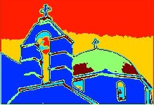
Fig. 1. (a) Original Berkeley image (n0 118035 )
The texture features of the original image shown in fig.1 (a) are calculated using Algorihm 1. The resulting feature vector is then nonlinearly reduced. Since we have used multiresolu- tion method the input image is down sampled. Nonlinearly dimensionality reduced output obtained after convergence of the conjugate gradient at coarser level is shown in fig. 1 (b). Final low-dimensional output obtained after interpolation and optimization at finer level is shown in fig. 1 (c). This low- dimensional feature vector is given as input to the clustering algorithm. FCM performs the segmentation and final seg- mented result is shown in fig. 1 (d)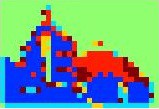
(b) Optimized low-dimensional image at coarser level
(c) Low-dimensional representation of original image

(d) Segmented image using FCM method
The segmentation algorithm was tested on the entire Berke- ley image database and some the segmented results are shown in fig. (2).

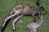
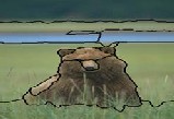

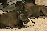
Fig. 2 Examples of segmentation results
For quantitative verification we have calculated probability rand index (PRI), variation of information (VoI), global con- sistency measure (GCE) and boundary displacement error (BDE) and compared with existing segmentation methods.
IJSER © 2013 http://www.ijser.org
International Journal of Scientific & Engineering Research, Volume 4, Issue 8, August-2013 1852
ISSN 2229-5518
The results are listed in table 1.
TABLE 1
PERFORMANCE COMPARISON
Algorithms | PRI | VoI | GCE | BDE |
Humans | .875 | 1.1040 | .0797 | 4.994 |
Multiresolution reduction model and FCM based segmentation | .756 | 2.464 | .1767 | 9.4211 |
Mean-Shift | .7550 | 2.477 | .2598 | 9.7001 |
NCuts | .7229 | 2.6647 | .1895 | 9.9497 |
From the table we can analyse that our method is superior to other listed methods in terms of all of the four performance measures.
In this paper a new method has been introduced for perform- ing color image segmentation of high dimensional data. Large scale dimensionality reduction problems can be overcome by using multiresolution reduction model. Low-dimensional rep- resentation of the texture feature vector of the input image is obtained by this algorithm. This detextured image can be rep- resented as a three channel image and can be exploited in the segmentation technique. For segmentation Fuzzy c-Means soft clustering method is used which produces better segmented results compared to hard segmentation techniques.
[1] M. Mignotte, “Segmentation by fusion of histogram-based K-means clusters in different color spaces,” IEEE Trans. Image Process., vol. 17 no. 5, pp. 780-787, May 2008
[2] D.E. Ilea and P.F. Whelan , “CTex- An adaptive unsupervised seg-
mentation algorithm on color-texture coherence,” IEEE Trans. Image
Process., vol. 17 no. 10, pp. 1926-1939, Oct 2008
[3] A.Y. Yang, J. Wright, S. S. Sastry, and Y. Ma, “Unsupervised segmen- tation of natural images via lossy data compression,”Comput. Vis. Im-
age Understand, vol. 110, no.2, pp. 212-225, May 2008
[4] J. Shi and J. Malik, “Normalized cuts and image segmentation,” IEEE Trans. Pattern Anal. Mach. Intell., vol. 22, no. 8, pp. 888-905, Aug.2000
[5] P. F. Felzenszwalb and D. P. Huttenlocher, “Efficient graph-based image segmentation,” Int. J.Comput. Vis. , vol. 59, no.2, pp. 161-181, Sep.2004
[6] R. Hedjam and M. Mignotte, “A hierarchical graph-bsed Markovian clustering approach for the unsupervised segmentation of textured color images,” in Proc. IEEE Int. Conf. Image Process., Cairo, Egypt, Nov. 2009, pp. 1365-1368
[7] S. P. Chatzis and G. Tsechpenakis, “The infinite hidden Markov ran-
dom field model,” IEEE Trans. Neural Ntew., vol. 21, no.6, pp. 1004-
1014, Jun.2010
[8] Q. Luo and T. M. Khoshgoftaar, “Unsupervised multiscale color image segmentation based on MDL principle,” IEEE Trans. Image Process., vol. 15, no. 9, pp. 2755-2761, Sep. 2006
[9] M. Krninidis and I. Pitas, “Color texture segmentation based on the modal energy of deformable surfaces,” IEEE Trans. Image Process., vol. 18, no. 7, pp. 1613-1622, Jul. 2009
[10] I. Mecimore and C. D. Creusere, “Unsupervised bitstream based segmentation of images,” in Proc. 5th IEEE Signal Process. Educ. Work- shop Dig. Signal Process., Workshop, Marco Island, FL, Jan. 2009,pp. 643-
647
[11] K. K. Bhoyar and O. G. Kakde, “Color image segmentation based on JND color histogram,” Int. J. Image Process., vol. 3, no. 6,pp. 282-293, Jan. 2010
[12] Y. Deng and B. S. Manjunath, “Unsupervised segmentation of color
texture regions in images and video,” IEEE Trans. Pattern Anal. Mach. Intell., vol, 23, no. 8, pp. 800-810, Aug. 2001
[13] S. C. Zhu and A. Yuille, “Region competition: Unifying snakes, re-
gion growing, and Bayes/MDL for multiband image segmentation,”
IEEE Trans. Pattern Anal. Mach. Intell., vol.18, no. 9, pp. 884-900, Sep.
1996
[14] S. R. Rao, H. Mobahi, A. Y. Yang, S. S. Sastry, and Y. Ma, “Natural image segmentation with adaptive texture and boundary encoding,” in Proc. Asian Conf. Comput. Vis., Part 1, LNCS 5994. Sep 2009, pp.
135-146
[15] H. Du, H. Qi, X. Wang, and R. Ramanath, “Band selection using in- dependent component analysis for hyperspectral image processing,” in Proc. 32nd Appl. Imagery Pattern Recog. Workshop, Washington D. C., Oct. 2003, pp. 93-98
[16] B. Scholkopf, A. Smola, K. R. Muller, “Kernel principal component analysis,”in advances in kernel methods-support vector learning,
1999, MIT press, Cambridge, MA, USA, 327-352
[17] S. T. Roweis and L. K. Saul, “Nonlinear dimensionality reduction using local linear embedding,” Science, vol. 290, no. 5500, pp. 2323-
2326, Dec. 2000
[18] J. B. Tenenbaum, v. de Silva, and J. C. Langford, “A global geometric frame work for nonlinear dimensionality reduction,” Science, vol.
290, no. 5500, pp. 2319-2323, Dec. 2000
[19] A. Mohan, G. Sapiro, and E. Bosh, “Spatially coherent nonlinear di- mensionality reduction and segmentation of hyperspectral images,” IEEE Geosci. Remote Sens. Lett., vol. 4,no. 2, pp.206-210, Apr. 2007
[20] A. Goh and R. Vidal, “Segmenting motions of different types by unsupervised manifold clustering,” in Proc. IEEE Conf. Comput. Vis. Pattern Recog., Minneapolis, MN, Jun. 2007, pp. 1-6
[21] Mikhail Belkin and Partha Niyogi, “Laplacian eigenmaps and spec-
tral techniques for embedding and clustering,” advances in neural in- formation processing systems 14, 2001, pp. 586-691, MIT Press
[22] D. Donoho and C. Grimes, “Hessian eigenmaps: Loacally linear em-
IJSER © 2013 http://www.ijser.org
International Journal of Scientific & Engineering Research, Volume 4, Issue 8, August-2013 1853
ISSN 2229-5518
bedding techniques for high dimensional data,” Proc. Natl. Acad. Sci. USA, May 2003, pp. 5591-5596
[23] Z. Zhang and J. Wang, “MLLE:Modified locally linear embedding using multiple weights”
[24] E. W. Dijkstra, “A not on two problems in connection with graphs,”
Numer. Math., vol. 1, no. 1, pp 269-271, Dec. 1959
[25] T. F. Cox and M. A. A. Cox, “Multidimensional scaling”London.
U.K., Chapman & Halll. 1994
[26] G. Young and A. Householder, “Discussion of a set of points in terms of their mutual distances,” Psychometrika, vol. 3, no. 1, pp. 19-
22, Mar. 1938
[27] W. S. Torgerson, “Multidimensional scaling: J. Theory and method,”
Psychometrika, vol. 17, no. 4, pp. 401-419, Dec. 1952
[28] C. Faloutsos and K. L. Lin, “Fastmap: A fast algorithm for indexing, data mining and visualization of traditional and multimedia da- tasets,” in Proc. ACM SIGMOD Int. Conf. Manage. Data. San Jose, CA, May 1995, pp. 163-174
[29] J. T. L. Wang, X. Wang, K. Lin, D. Shasha, B. A. Shapiro, and K.
Zhang, “Evaluating a class of distance mapping algorithms for data mining and clustering,” Dept. Math., Stanford University, Stanford, CA, Tech. Rep. , Jun. 2004
[30] V. de Silva and J. D. Tenenbaum,”Sparse multidimensional scaling using landmark points, ” Dept. Math., Stanford University, Stanford, CA, Tech. Rep. Jun. 2004
[31] J.C. Platt, “Fastmap, Metricmap and landmark MDS are all Nystrom algorithms,” in Proc. 10th int. Workshop Artif. Intell. Stat., Jan. 2005, pp.
261-268
[32] M. Mignotte,”MDS-based multiresolution nonlinear dimensionality reduction model for color image segmentation,” in IEEE Trans. Neural Netw., vol. 22, no. 3, March 2011
[33] Bezdek, J.C.: pattern recognition with fuzzy objective function algo-
rithms, New York, Plenum Press, 1981.
IJSER © 2013 http://www.ijser.org