In this section, the mathematical background of the scattering features used for image classification is
International Journal of Scientific & Engineering Research, Volume 5, Issue 7, July-2014
ISSN 2229-5518
Classification of hyperspectral images using scattering transform
Ashitha P S, V Sowmya, K P Soman
315
Abstract- In this paper, we applied scattering transform approach for the classification of hyperspectral images. This method integrates features, such as the translational and rotational invariance features for image classification. The classification of hyperspectral images is more challenging because of the very high dimensionality of the pixels and the small number of labelled examples typically av ailable for learning. The scattering transform technique is validated with two standard hyperspectral datasets i .e, SalinasA_Scene and Salinas_Scene. The experimental result analysis proves that the applied scattering transform method provides high classification accuracy of 99.35% and
89.30% and kappa coefficients of 0.99 and 0.88 for the mentioned hyperspectral image d ataset respectively.
—————————— ——————————
he classification of hyperspectral images become challenging since the dimension of the images is considerable for the classification algorithms. The
high dimensionality of the data/pixels and the small number of labeled samples typically available for the learning of the classifier is also a fact which leads the classification a challenging task. To overcome this problem, the method of feature extraction is introduced before training the classifier. These extracted features of the images are given for the learning of the classifier, so that the overall performance of the classifier increases to a great extent. Many supervised and non-supervised methods are proposed earlier for the classification of the hyperspectral images by reducing the dimension of the image [1].
The classification of hyperspectral images is done using Optimized Laplacian SVM with Distance Metric Learning method in [2]. Optimized Laplacian SVM are developed for semisupervised hyperspectral image classification, by introducing with Distance Metric Learning instead of the traditional Eucliden distance which are used in the existing LapSVM. In the given reference [3] the kernel method is applied to extend NWFE to kernel-based NWFE (KNWFE). The experimental results of three hyperspectral images show that KNWFE can have the highest classification accuracy under three training- sample-size conditions.
————————————————
Ashitha P S is currently pursuing masters degree program in Remote sensing and wireless sensor networks,at Amrita Vishwa Vidyaeetham,Tamilnadu. E-mail: 2k7ashi@mail.com
V Sowmya, Assistant professor in the Centre for Excellence in Computational Engineering and Networking, Amrita Vishwa Vidyaetham, Tamilnadu. She is currently pursuing her Phd in Image processing.
Dr.K P Soman, Head of the Centre for Excellence in Computational Engineering and Networking, Amrita Vishwa Vidyaetham, Tamilnadu.
Experimental results also show that the performance of KNWFE is not consistently better than those of the other methods under small number of features and training sample condition. A new method for hyperspectral image classification is proposed in [4] based on manifold learning algorithm. A new Laplacian eigen map pixels distribution flow (LEPD-Flow) is proposed for hyperspectral image analysis, in which, a new joint spatial-pixel characteristic distance (JSPCD) measure is constructed to improve the accuracy of classification. In this proposed work, a new method for the classification of the hyperspectral images in which the translational and rotational invariance features of each pixel in the image is extracted by applying the scattering transform to the image. These extracted features give a high accuracy of classification for Salinas_Scene and SalinasA_Scene hyperspectral image datasets.
This paper is organized as follows: The diffusion
technique used in this work is described in sect 2. Sect.3 provides the description of the proposed feature extraction method. Sect.4 describes the classifier algorithm used. A brief note on the dataset used in this work is given in sect.5. Experimental results are presented in sect.6, followed by the conclusion.
Perona Malik diffusion also called anisotropic diffusion is a technique for reducing the image noise, without removing the significant parts of the image. It preserves the information significant for the interpretation of the image. The resulting image is obtained by the convolution between the image and a two dimensional isotropic Gaussian filters. This is a nonlinear and space variant transformation of the image [5]. Each successive image in the family is computed by an iterative process where a relatively simple set of computations are performed and the process can be repeated until the required degree of smoothing is obtained [6]. The proposed method iterated with a number of values of
IJSER © 2014
International Journal of Scientific & Engineering Research, Volume 5, Issue 7, July-2014
ISSN 2229-5518
316
iterations to find out the best value for sufficient smoothening. The two datasets are iterated several times and the resulting pre-processed diffused image is taken further for feature extraction step.
insensitive to local translation and reduce the variability of these coefficients their complex phase is removed by a modulus and it is averaged by J which are the scattering coefficients represented by Eq (1).![]()
In this section, the mathematical background of the scattering features used for image classification is![]()
![]()
x * j , * j ,
*J
(1)
presented. Scattering transform [7] is used to extract the features of hyperspectral images used in this work. This method is efficient for extracting features based on the translation, rotational and convolutional invariance of the image pixels. The scattering transform is implemented in
Scat Net using the scat function [8]. This function can be
A scattering vector computed with a cascade of
convolutions and modulus operators over m+1 layers,
like in convolution network architecture is given in Eq
(2).
used to calculate several types of scattering transforms by varying the linear operators supplied to it.
x(n) x *J
(2J n)
![]()
![]()
J
![]()
![]()
The features extracted for classification need to be invariant with respect to the transformations which do![]()
x * j ,
x * j , *J (2 n)
(2)
J
not affect our ability to recognize. Scattering transforms build invariant, stable and informative representations through a non-linear, unitary transform, which delocalizes the information into scattering decomposition![]()
![]()
x * j , * j ,
![]()
![]()
![]()
x * j , * j ,
*J (2 n)
paths. They are computed with a cascade of wavelet modulus operators, and correspond to a convolutional
Scattering propagator U J![]()
![]()
applied to ‗x‘ computes each
network where filter coefficients are given by a wavelet
U 1
x x
1
and gives the output features
operator [9].
In particular, as the scale of the low pass window grows,
SJ x x
. Applying
U J to each
U 1 x
and after an appropriate renormalization, the scattering
computes all
U 1 , 2 x and output
transform converges into a translation invariant integral transform, defined on an uncountable path space [10].
SJ 1 U
1
is given. Applying U J iteratively
The resulting integral transform shares some properties
with the Fourier transform; in particular, signal decay can
be related with the regularity on the integral scattering domain.
The translational and rotational invariant features of an image ‗x‘ is obtained by averaging the image over all translations ‗j‘ and rotations ‗ ‘ . i.e., the convolution
to each U p x gives the output features and computes
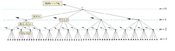
the next path layer. The three layers of coefficients obtained by applying the scattering transform to an image ‘x‘ is shown in fig 1.
with the low ass filter
J .The high frequencies
eliminated in![]()
x *
j1 ,1
![]()
*J by the convolution with J
are recovered by convolution with wavelets
x * j1 ,1 | * at scales 2 j2 2J . To become j2 , 2 | |
Fig 1, Scattering Convolution Network [9] |
IJSER © 2014
International Journal of Scientific & Engineering Research, Volume 5, Issue 7, July-2014
ISSN 2229-5518
317
The scattering transform selects the discriminating features and a classification scheme must be identified to exploit them. This section discusses the support vector machine (SVM) classification algorithm used in this work. A classification task usually involves separating data into training and testing sets [11]. Each instance in the training set contains one target value and several attributes. The goal of SVM is to produce a model (based on the training data) which predicts the target values of the test data. The reason for opting SVM classifier is mainly to overcome the local minima problem which is generally faced in neural network classifier. Furthermore, most of the problems are modeled using Gaussian distribution function which may not be the case in most of the real-life applications.
Given a training set of instance-label pairs (xi, yi), i=1,...,l where xi Rn and y {1,-1}l. The objective function and kernel functions are given in Eq (3) and Eq (4) [12]. The support vector machine require the solution of the
following optimization problem:
available only as at-sensor radiance data. It includes vegetables, bare soils, and vineyard fields and its ground truth contains 16 classes. The next dataset used in this work is SalinasA_Scene. A small sub scene of Salinas image, denoted SalinasA , is usually used. It comprises
86×83 pixels located within the same scene at [samples,
lines] = [591-676, 158-240] and includes six classes [15].
Accuracy assessment is an essential metric for image classification to determine the performance of the classification technique used. The accuracy assessment reflects the difference between the classified data and the ground truth data [16]. Classification accuracy in case of hyperspectral image can be statistically measured using various parameters. These statistical measures can be easily obtained from the Confusion Matrix or the Classification Error Matrix (also known as contingency table)[2]. The overall accuracy is calculated as the total number of correctly classified pixels divided by the total number of test pixels. The kappa statistics is the most popular technique for comparing different classifiers. To quantify the agreement of classification, the kappa
min
1 l![]()
wT w C
coefficient can be used. The mathematical equation for
w,b, 2
T
i 1
calculating the overall accuracy and kappa coefficient is
given by Eq (5) and Eq (6) [16].
Subject to
yi (w (xi ) b) 1 i ,
i 0
(3)![]()
Overall Accuracy Total number of correctly classified pixels (5)
Total number of pixels
K (x , x ) (x )T (x ) is called the kernel function.
kappa coefficient(k ) (N * A B) / (N 2 B)
(6)
K ( x , x ) (x T x
i j i j
r)d , 0
Where ‗N‘ is the total number of pixels, ‗A‘ is the number
(4) of correctly classified pixels (Sum of diagonal elements in
the confusion matrix), ‘B‘ is the sum of product of row
and column total in confusion matrix.
If the number of features is large, one may not need to
map to a higher dimensional space. That is, the nonlinear
mapping does not improve the performance [13]. Using
the linear or polynomial kernel is good enough, and the
one only searches for the control parameter ‗C‘. Here in this work, LIBSVM [14] which is an integrated software for support vector classification, (C-SVC, nu-SVC), regression (epsilon-SVR, nu-SVR) and distribution estimation (one-class SVM) is used for the classification.
Two standard datasets namely Salinas_Scene and SalinasA_Scene are used to analyse the performance of the scattering transform technique for image classification. The first dataset, Salinas_Scene is collected by the 224-band Airborne Visible Infrared Imaging Spectrometer(AVIRIS) sensor over Salinas Vally, California, and is characterized by high spatial resolution (3.7-meter pix). The area covered comprises 512 lines by
217 samples and the bands : [108-112], [154-167], 224 are rejected as water absorption bands. This image is
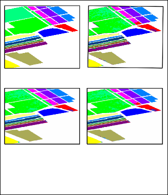
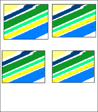
The best value for control parameter ‗C‘ and gamma is fixed by randomly selecting 80% of the pixels for training and the remaining 20% for testing. The same procedure is iterated five times for all different possible combinations of ‗C‘ and gamma (C=10,100,500 and gamma=0.1, 1, 10) for each dataset. Once the ‗C‘ and gamma value is fixed, the experiment is performed on each dataset with 40% of the pixels for training and the remaining 60% for testing. The experimental results are evaluated with the metric called classification accuracy and kappa coefficient. This procedure is repeated for three different kernels i.e, linear, polynomial and RBF kernels. The classification accuracy and kappa coefficient obtained for different kernels for Salinas_Scene and SalinasA_Scene is given in table 1. The classification map of original ground truth data and the output of the applied scattering transform for three different kernels for Salinas_Scene and SalinasA_Scene hyperspectral image dataset is shown in the fig 2 and fig 3 below.
IJSER © 2014
International Journal of Scientific & Engineering Research, Volume 5, Issue 7, July-2014
ISSN 2229-5518
318
TABLE 1 CLASSIFICATION ACCURACY AND KAPPA COEFFICIENT FOR THREE DIFFERENT KERNELS FOR HYPERSPECTRAL IMAGE
DATASET
C | Gamma | Linear Kernel | Polynomial Kernel | RBF Kernel | ||||
C | Gamma | Accuracy (%) | Kappa | Accuracy (%) | Kappa | Accuracy (%) | Kappa | |
SalinasA_Scene | 500 | 0.1 | 98.50 | 0.98 | 99.35 | 0.99 | 98.49 | 0.98 |
Salinas_Scene | 500 | 1 | 86.35 | 0.84 | 89.30 | 0.88 | 88.87 | 0.87 |
(a) (b)
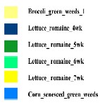
(c) (d) Fig 2, Classification map of SalinasA_Scene
(a) Original Ground truth (b) Linear kernel classifier
(c) Polynomial kernel classifier (d) RBF kernel classifier
(a) (b)
(c) (d)
(c) (d)
Fig 3, Classification map of Salinas_Scene
(a) Original Ground truth (b) Linear kernel classifier
(c) Polynomial kernel classifier (d) RBF kernel classifier.

IJSER © 2014
International Journal of Scientific & Engineering Research, Volume 5, Issue 7, July-2014
ISSN 2229-5518
319
Features are extracted using scattering transform and the classification is done using support vector machine. The translation and rotation invariant features of an image are extracted using the scattering transform which improves the hyperspectral image classification accuracy to a great extent. The accuracy obtained by this method for SalinasA_Scene dataset is 99.35% for polynomial kernel with a kappa coefficient of 0.99. The accuracy and kappa coefficient for Salinas_Scene dataset is 89.30% and
0.88 for polynomial kernel. The same procedure can be
repeated for different wavelet filters used in the
scattering transform for feature extraction. This may lead to the high classification accuracy for various other image datasets.
[1] Ping Zhong, Member, IEEE, And Runsheng Wang, ―Learning Conditional Random Fields For Classification Of Hyperspectral Images‖ IEEE Transactions On Image Processing, Vol. 19, No. 7, July 2010.
[2] Yanf eng gu, member, IEEE, and kai feng, ―Optimized
laplacian svm with distance metric Learning for hyperspectral image classification‖ IEEE Journal Of Selected Topics In Applied Earth Observations And Remote Sensing, Vol. 6, No. 3, June2013.
[3] Bor-Chen Kuo,Cheng-Hsuan Li and Jinn-Min Yang, ―Kernel
Nonparametric Weighted Feature Extraction for Hyperspectral Image Classification‖ IEEE Transactions On Geoscience And Remote Sensing, Vol. 47, No. 4, April 2009.
[4] Biao Hou, Member, IEEE, Xiangrong Zhang, Member, IEEE, Qiang Ye, and Yaoguo Zheng, ―A Novel Method for Hyperspectral Image Classification Based on Laplacian Eigenmap Pixels Distribution-Flow‖ IEEE Journal Of Selected Topics In Applied Earth Observations And Remote Sensing, Vol. 6, No. 3,June 2013.
[5] Guo W. Wei, Member, IEEE, ―Generalized Perona–Malik Equation for Image Restoration‖ IEEE Signal Processing Letters, Vol. 6, No. 7, July 1999.
[6] Kavitha Balakrishnan, Sowmya V., Dr. K.P. Soman, ―Spatial Preprocessing for Improved Sparsity Based Hyperspectral Image Classification‖, International Journal of Engineering Research & Technology (IJERT) Vol. 1 Issue 5, July – 2012
ISSN: 2278-0181.
[7] Joan Bruna Estrach, CMAP, Ecole Polytechnique, ―Scattering Representations for Recognition‖ PhD thesis Submitted November 2012.
[8] http://www.di.ens.fr/data/software/scatnet/
[9] Joan Bruna and Stephane Mallat, ―Invariant Scattering Convolution Networks‖ CMAP, Ecole Polytechnique, Palaiseau, France.
[10] Huajuan Wu, Mingjun Li ,Mingxin Zhang, Jinlong Zheng and Jian Shen, ―Texture Segmentation via Scattering
Transform‖ International Journal of Signal Processing, Image
Processing and Pattern Recognition Vol. 6, No. 2, April, 2013. [11] Gustavo Camps-Valls, Member, IEEE, and Lorenzo Bruzzone,
Senior Member, IEEE, ―Kernel-Based Methods for
Hyperspectral Image Classification‖ IEEE Transactions On
Geoscience And Remote Sensing, Vol. 43, No. 6, June 2005. [12] K P Soman, R Loganathan, V Ajay, ― Machine learning with
SVM and other kernel methods‖, published on 2009 by PHI
Learning Private Limited, New Delhi.
[13] Chih-Wei Hsu, Chih-Chung Chang, and Chih-Jen Lin, ―A Practical Guide to Support Vector Classication‖ Department of Computer Science National Taiwan University, Taipei 106, Taiwan.
[14] http://www.csie.ntu.edu.tw/~cjlin/libsvm/
[15]http://www.ehu.es/ccwintco/index.php/Hyperspectral_Rem ote_Sensing_Scene.
[16] Ryuei Nishii,Member, IEEE,and Shojiro Tanaka,Member, IEEE, ―Accuracy and Inaccuracy Assessments in Land-Cover Classification‖ IEEE Transactions On Geoscience And Remote Sensing, Vol. 37, No. 1, January 1999.
IJSER © 2014