International Journal of Scientific & Engineering Research, Volume 4, Issue 12, December-2013 2063

ISSN 2229-5518

COVARIENCE ESTIMATION AND PERFORMANCE OF SATELLITE IMAGINARY DATA USING SMT

G SRI HARSHINI, J KRISHNA CHAITANYA

Abstract: Covariance estimation for high dimensional vectors is a classically difficult problem in statistical analysis and machine learning. In this paper, we propose a maximum likelihood (ML) approach to covariance estimation, which employs a novel sparsity constraint. More specifically, the covariance is constrained to havean Eigen decomposition which can be represented as a sparse matrix transforms (SMT). The SMT is formed by a product of pairwise coordinate rotations knownas Givens rotations. Using this framework, the covariance can be efficiently estimated using greedy minimization of the log likelihood function, and the number of Givens rotations can be efficiently computed using a cross-validation procedure. The resulting estimator is positive definite and well-conditioned even whenthe sample size is limited. Experiments on standard hyper-spectral data sets show that the SMT covariance estimate is consistently more accurate than both traditional shrinkage estimates and recently proposed graphical lasso estimates for a variety of different classes and sample sizes.

Keywords —Covariance estimation, Eigen-image analysis, hyper spectral data, maximum likelihood estimation, sparse matrix transform, Compressed

sensing, Linear Mixing Model

---------------- ♦ ------------------

IJSER

1. INTRODUCTION

As the capacity to measure and collect data increases, high dimensional signals and systems have become much more prevalent. Medical imaging, remote sensing, internet communications, and financial data analysis are just a few examples of areas in which the dimensionality of signals is growing explosively, and leading to an unprecedented quantity of information and potential knowledge. However, this growth also presents new challenges in the modeling and analysis of high dimensional signals (or data). In practice, the dimensionality of signals (p) often grows much faster than the number of available observations (n). The resulting “smalln, largep ” scenario [1] tends to break the basic assumptions of classical statistics and can cause conventional estimators to behave poorly. In fact, Donoho makes the very reasonable claimp>n that is in fact the more generic case in learning and recognition problems [2]; so, this “curse of dimensionality” [3], [4] represents a very fundamental challenge for the future.
A closely related problem to the curse of dimensionality is the super-linear growth in computation that can occur with
classical estimators as p grows large. For example, classical
methods such as singular value decomposition (SVD) and eigen-analysis depend on the use of dense p x p transformations that can quickly become intractable to apply (or estimate) as the dimension grows. Therefore, the modeling and analysis of high dimensional signals pose a fundamental challenge not only from the perspective of inference, but also from the perspective of computation. A fundamental step in the analysis of high dimensional signals is the estimation of the signal’s covariance. In fact, an accurate estimate of signal covariance is often a key step in detection, classification, and modeling of high dimensional signals, such as images [5], [6]. However, covariance estimation for high dimensional signals is a classically difficult problem because the number of coefficients in the covariance grows as the dimension squared [7], [8]. In a typical application, one may measure versions of n a dimensional vector; so if n<p, then the sample covariance matrix will be singular with p-n eigen values equal to zero.
Over the years, a variety of techniques have been proposed for computing a nonsingular estimate of the covariance. For example, shrinkage and regularized covariance estimators

International Journal of Scientific & Engineering Research, Volume 4, Issue 12, December-2013 2064

ISSN 2229-5518

are examples of such techniques. Shrinkage estimators are a
widely used class of estimators which regularize the covariance matrix by shrinking it toward some positive definite target structures, such as the identity matrix or the diagonal of the sample covariance [9]–[13]. In this paper, we propose a new approach to covariance estimation, which is based on constrained maximum likelihood (ML) estimation of the covariance from sample vectors [14]. In particular, the covariance is constrained to be formed by an eigen-transformation that can be represented by a sparse matrix transform (SMT) [15]; and we define the SMT to be an orthonormal transformation formed by a product of pairwise coordinate rotations known as Givens rotations [16]. Using this framework, the covariance can be efficiently estimated using greedy maximization of the log likelihood function, and the number of Givens rotations can be efficiently computed using a cross-validation procedure. The estimator obtained using this method is generally positive definite and well-conditioned even when the
sample size is limited.
In order to validate our model, we perform experiments using simulated data, standard hyper-spectral image data, and face image data sets. We compare against both traditional shrinkage estimates and recently proposed graphical lasso estimates. Our experiments show that, for these examples, the SMT-based covariance estimates are consistently more accurate for a variety of different classes and sample sizes. Moreover, the method seems to work particularly well for estimating small eigenvalues and their associated eigenvectors; and the cross-validation procedure used to estimate the SMT model order can be implemented with a modest increase in computation.

2. SYSTEM DESIGN MODEL

2.1 Covariance estimation for high dimensional vectors

In the general case, we observe a set of n vectors, y1; y2; ; y n , where each vector, y i , is p dimensional. Without loss of

IJSEgenerality, weRassume y i has zero mean. We can represent

Due to its flexible structure and data-dependent design, the

SMT can be used to model behaviors of various kinds of natural signals. We will show that the SMT can be viewed as a generalization of both the classical fast Fourier transform (FFT) [17] and the orthonormal wavelet transforms. Since these frequency transforms are commonly used to de-correlate and therefore model stationary random processes, the SMT inherits this valuable property.We will also demonstrate that autoregressive (AR) and moving average (MA) random processes can be accurately modeled by a low-order SMT. However, the SMT is more expressive than conventional frequency transforms because it can accurately model high dimensional natural signals that are not stationary, such as hyper-spectral data measurements. In addition, it is shown that the SMT covariance estimate is invariant to permutations of the data coordinates; a property that is not shared by models based on the FFT or wavelet transforms. Nonetheless, the SMT model does impose a substantial sparsity constraint through a restriction in the number of Givens rotations. When this sparsity constraint holds for real data, then theSMT model can substantially improve the accuracy of covarianceestimates; but conversely if the eigen-space of the random process has no structure, then the SMT model
provides no advantage [18].
this data as the following p n matrix
𝑌 = [𝑌1 ; 𝑌2 ; ; 𝑌𝑛 ]: (1)
If the vectors Y1 are identically distributed, then the sample
𝑆 = 𝑛 𝑌 𝑌𝑡 ; (2)
And Sis an unbiased estimate of the true covariance matrix1
𝑅 = 𝐸 𝑦1 𝑦𝑡 = 𝐸[𝑆]
While S is an unbiased estimate of R it is also singular when
n < p. This is a serious deciency since as the dimension p grows, the number of vectors needed to estimate R also grows. In practical applications, n may be much smaller than p which means that most of the eigen values of R are erroneously estimated as zero.
A variety of methods have been proposed to regularize the estimate of R so that it is not singular. Shrinkage estimators are a widely used class of estimators which regularize the covariance matrix by shrinking it toward some target structures [4, 5, 6, 7, 8]. Shrinkage estimators generally have the form, where is some positive de nite matrix. Some popular choice for
R = D + (1)S D
D are the identity matrix (or its scaled version) [5, 8, 6] and the diagonal entries of S, i.e. diag(S) [5, 8]. In both cases, the shrinkage intensity can be estimated using cross-validation or boot-strap methods.

International Journal of Scientific & Engineering Research, Volume 4, Issue 12, December-2013 2065

ISSN 2229-5518

Recently, number methods have been proposed for regularizing the estimate by making either the covariance or its inverse sparse [9, 10, 14]. For example, the graphical lasso method enforces sparsity by imposing an L1 norm constraint on the inverse covariance [14]. Banding or thresholding can also be used to obtain sparse estimates of the covariance.

2.2 Maximum likelihood covariance estimation

Our approach will be to computer a constrained maximum likelihood(ML)estimate of the covariance R, under the modeling assumption that Eigen vectors of R may be represented as a sparse matrix transform(SMT). So we first
decompose R as
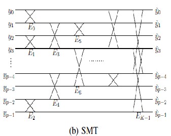
the organization of the butterflies in an SMT is unstructured, and each butterfly can have an arbitrary rotation angle k. This more general structure allows anSMT to implement a larger set of orthonormal transformations. In fact, the SMT can be used torepresent any orthonormal wavelet transform because orthonormal wavelets can be factorized into aproduct of Givens rotations and delays [17].

𝑅 = 𝐸 𝐸𝑡 ;
Where E is the orthonormal matrix of eigenvectors and is
the diagonal matrix of eigenvalues.

Then we will estimate the covariance by maximizing the likelihood of the data Y subject to the constraint that E is an SMT. By varying the order, K , of the SMT, we may then reduce or increase the regularizing constraint on the covariance.

2.3 ML estimation of eigenvectors using SMT model

The ML estimate of E can be improved if the feasible set of
eigenvector transforms, , can be constrained to a subset of all possible orthonormal transforms. By constraining, we effectively regularize the ML estimate by imposing a model. However, as with any model-based approach, the key is to select a feasible set, , which is as small as possible while still accurately modeling the behavior of the data. Our approach is to select to be the set of all orthonormal transforms that can be represented as an SMT of order K [11]. More specifically, a matrix E is an SMT of order K if it can be written as a product of K sparse orthonormal matrices.
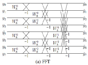
Figure 1 shows the flow diagram for the application of an SMT to a data vector y. Notice that each2D rotation, Ek, plays a role analogous to a .butterfly. used in a traditional
fast Fourier transform(FFT) [16]. However, unlike an FFT,

Figure 1: (a) 8-point FFT. (b) The SMT implementation, The SMT can be viewed as a generalization of FFT and orthonormal wavelets.

The model order, K, can be determined by a simple cross- validation procedure. After portioning the data into three subsets, K is chosen to maximize the average likelihood of the left-out subsets given the estimated covariance using the other two subsets. Once K is determined, the proposed covariance estimator is re-computed using all the data and the estimated model order.

International Journal of Scientific & Engineering Research, Volume 4, Issue 12, December-2013 2066

ISSN 2229-5518

The SMT covariance estimator obtained as above has some interesting properties. First, it is positive definite even for the limited sample size n < p. Also, it is permutation invariant, that is, the covariance estimator does not depend on the ordering of the data. Finally, the eigen decomposition Et y can be computed very efficiently by applying the K sparse rotations in sequence.

3. SIMULATION RESULTS

The effectiveness of the SMT covariance estimation procedure depends on how well the SMT model can capture the behavior of real data vectors. Therefore in this section, we compare the effectiveness of the SMT covariance estimator to commonly used shrinkage and graphical lasso estimators. We do this comparison using

hyper-spectral remotely sensed data as our high
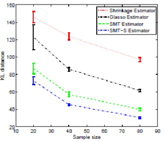
of the grass pixels, and Fig. 2(c) shows multivariate Gaussian vectors that were generated using the measured sample covariance for the grass class.

Gaussian case: First, we compare how different estimators perform when the data vectors are samples from an ideal multivariate Gaussian distribution. To do this, we first generated zero mean multivariate vectors with the true covariance for each of the five classes. Next we estimated the covariance using the four methods, SMT covariance estimation and the three shrinkage methods. In order to determine the effect of sample size, we also performed each experiment for a sample size of n = 80, 40, and 20. Every experiment was repeated 10 times.

dimensional data vectors. The hyper-spectral data we use is available with the recently published book [13]. Figure 2(a) shows a simulated color IR view of an airborne hyper- spectral data flight line over the Washington DC Mall. The sensor system measured the pixel response in 191 effective bands in the 0.4 to 2.4 m region of the visible and infrared spectrum. The data set contains 1208 scan lines with 307 pixels in each scan line. The image was made using bands
60, 27 and 17 for the red, green and blue colors,
respectively.
The data set also provides ground truth pixels for five classes designated as grass, water, roof, street, and tree. In Figure 2, the ground-truth pixels of the grass class are outlined with a white rectangle. For each class, we computed the “true” covariance by using all the ground truth pixels to calculate the sample covariance. The covariance is computed by rst subtracting the sample mean vector for each class, and then computing the sample covariance for the zero mean vectors. The number of pixels for the ground-truth classes of grass, water, roof, street, and tree are 1928, 1224, 3579, 416, and 388, respectively. In each case, the number of ground truth pixels was much larger than 191, so the true covariance matrices are nonsingular, and accurately represent the covariance of the hyper-
spectral data for that class. Figure 2(b) shows the spectrum

Figure 2: Kullback-Leibler distance from true distribution versus sample size for various classes: Gaussian case.

In order to get an aggregate assessment of the effectiveness of SMT covariance estimation, we com-pared the estimated covariance for each method to the true covariance using the Kull back-Leibler (KL) distance [15]. The KL distance is a measure of the error between the estimated and true distribution. Figure 2 show plots of the KL distances as a function of sample size for the four estimators. The error bars indicate the standard deviation of the KL distance due to random variation in the sample statistics. Notice that the SMT shrinkage (SMT-S) estimator is consistently the best of the four.

International Journal of Scientific & Engineering Research, Volume 4, Issue 12, December-2013 2067

ISSN 2229-5518

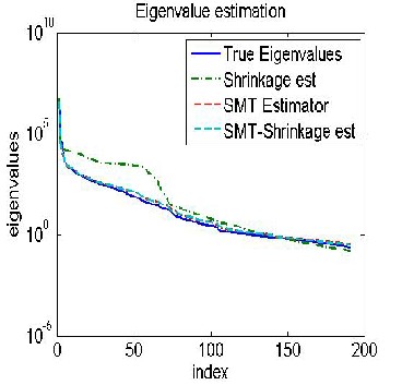
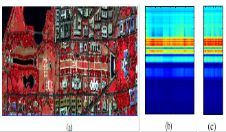
Figure 3: (a) simulated color IR view of an airborne hyper-spectral data over the Washington DCMall [13]. (b) Ground-truth pixel spectrum of grass that are outlined with the white rectangles ina). (c)

Synthesized data spectrum using the Gaussian distribution.

Figure 4(a) shows the estimated eigenvalues for the grass
class with n = 80. Notice that the eigenvalues of the SMT and SMT-S estimators are much closer to the true values than the shrinkage or glasso methods. Notice that the SMT estimator generates good estimates for the small
eigenvalues.This is because the SMT transform is a sparse

Figure 4: The distribution of estimated eigenvalues for the grass class with n = 80. (a) Gaussian case (b) Non-Gaussian case.

operator. In this case, the SIMT useJs an averageSof K = 495 ER
rotations, which is equal to K=p = 495=191 = 2:59 rotations
(or equivalently multiplies) per spectral sample.

Non-Gaussian case: In practice, the sample vectors may not

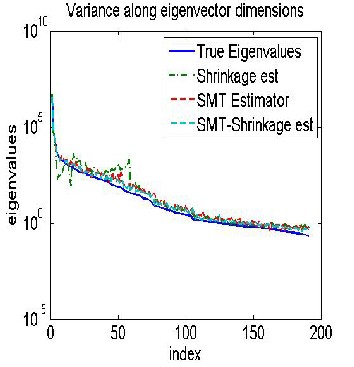
be from an ideal multivariate Gaussian distribution. In order to see the effect of the non-Gaussian statistics on the accuracy of the covariance estimate,we performed a set of experiments which used random samples from the ground truth pixels asinput. Since these samples are from the actual measured data, their distribution is not precisely Gaussian. Using these samples, we computed the covariance estimates for the five classes using thefour different methods with sample sizes of n = 80, 40, and 20.Plots of the KL distances for the non-Gaussian grass case2are shown in Figure 2; and Figure 4(b) shows the estimated eigenvalues for grass with n = 80. Note that the results are
similarto those found for the ideal Guassian case.

International Journal of Scientific & Engineering Research, Volume 4, Issue 12, December-2013 2068

ISSN 2229-5518

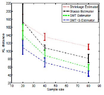
Figure 5: Kullback-Leibler distance from true distribution versus sample size for various classes: non-Gaussian case

[2] D. L. Donoho, “High-dimensional data analysis: The curses and blessingsof dimensionality,” in Math Challenges of the 21st Century. LosAngeles, CA: American Mathematical Society, Aug. 8, 2000.

[3] R. E. Bellman, Adaptive Control Processes. Princeton, NJ:

PrincetonUniv. Press, 1961.

[4] A. K. Jain, R. P. Duin, and J. Mao, “Statistical pattern recognition: Areview,” IEEE Trans. Pattern Anal. Mach. Intell., vol. 22, no. 1, pp.4–37, Jan. 2000.

[5] P. N. Belhumeur, J. P. Hespanha, and D. J. Kriegman, “Eigenfacesversus fisherfaces: Recognition using class specific linear projection,”IEEE Trans. Pattern Anal. Mach. Intell., vol. 19, no. 7, pp.

711–720,Jul. 1997.

[6] J. Theiler, “Quantitative comparison of quadratic covariance- basedanomalous change detectors,” Appl. Opt., vol. 47, no. 28, pp. F12– F26,2008.

[7] C. Stein, B. Efron, and C. Morris, “Improving the usual estimator of

anormal covariance matrix,” Dept. of Statistics, Stanford Univ.,

4. CONCLUSION

Report37, 1972.

IJSE[8] K. FukunagRa, Introduction to Statistical Pattern Recognition, 2nd

We have proposed a novel method for covariance estimation of high dimensional data. The new method is based on constrained maximum likelihood (ML) estimation in which the eigenvector transformation is constrained to be the composition of K Givens rotations. This model seems to capture the essential behavior of the data with a relatively small number of parameters. The constraint set is a K dimensional manifold in the space of orthonormal transforms, but since it is not a linear space; the resulting ML estimation optimization problem does not yield a closed form global optimum. However, we show that a recursive local optimization procedure is simple, intuitive, and yields good results. We also demonstrate that the proposed SMT covariance estimation method substantially reduces the error in the covariance estimate as compared to current state-of-the-art estimates for a standard hyper- spectral data set.

REFERENCES

[1] T. Hastie, R. Tibshirani, and J. Friedman, The Elements of

StatisticalLearning: Data Mining, Inference and Prediction, 2nd ed. NewYork:Springer, 2009.

ed.Norwell, MA: Academic, 1990.

[9] J. H. Friedman, “Regularized discriminant analysis,” J. Amer. Stat.Assoc., vol. 84, no. 405, pp. 165–175, 1989.

[10] J. P. Hoffbeck and D. A. Landgrebe, “Covariance matrix

estimationand classification with limited training data,” IEEE Trans. Pattern Anal.Mach. Intell., vol. 18, no. 7, pp. 763–767, Jul. 1996.

[11] M. J. Daniels and R. E. Kass, “Shrinkage estimators for

covariancematrices,” Biometrics, vol. 57, no. 4, pp. 1173–1184, 2001.

[12] O. Ledoit and M. Wolf, “A well-conditioned estimator for large- dimensionalcovariance matrices,” J. Multivar.Anal., vol. 88, no. 2, pp.365–411, 2004.

[13] J. Schafer and K. Strimmer, “A shrinkage approach to large-scale covariancematrix estimation and implications for functional genomics,”Stat. Appl. Genet.Molecular Biol., vol. 4, no. 1, 2005.

[14] G. Cao and C. Bouman, “Covariance estimation for high dimensionaldata vectors using the sparse matrix transform,” in Advances in NeuralInformation Processing Systems. Cambridge, MA: MIT Press, 2008,pp. 225–232.

[15] G. Cao, C. Bouman, and K. Webb, “Noniterative map

reconstructionusing sparse matrix representations,” IEEE Trans. Image

Process., vol.18, no. 9, pp. 2085–2099, Sep. 2009.

International Journal of Scientific & Engineering Research, Volume 4, Issue 12, December-2013 2069

ISSN 2229-5518

[16] W. Givens, “Computation of plane unitary rotations transforming ageneral matrix to triangular form,” J. Soc. Industrial Appl. Math., vol.6, no. 1, pp. 26–50, Mar. 1958.

[17] J. W. Cooley and J. W. Tukey, “An algorithm for the machine

calculationof complex Fourier series,” Math. Comp. , vol. 19, no. 90, pp.297–301, Apr. 1965.

[18] G. Cao, C. A. Bouman, and J. Theiler, “Weak signal detection in hyper-spectral imagery using sparse matrix transformation (SMT) covarianceestimation,” presented at the WHISPERS: First Workshop on Hyper-spectral Image and Signal Processing: Evolution in Remote Sensing,Grenoble, France, Aug. 2009.

IJSER