International Journal of Scientific & Engineering Research, Volume 4, Issue 7, July-2013
ISSN 2229-5518
CONSTRUCTION OF STRAIGHT LINE WALKING BEAM EIGHT BAR TRANSPORT MECHANISM
2135
1Mr. Ashish Kumar (Asst. Professor, Department of Mechanical Engineering, S.R.M University); Email:
ashish.k@ncr.srmuniv.ac.in. 2Ashish Kumar; Email: aksrivastava1991@gmail.com.
Abstract—This paper aims for the utilization of kinematic synthesis (type, dimensional and number) to fabricate a working physical model of an eight link transport mechanism. The mechanism to be developed in its simplest form would perform the function of transporting boxes/articles which are being fed onto two rails and are moved ahead one by one. The eight bar mechanism allows moving more than one article as compared to its four bar counterpart. Transport mechanisms generally move material and their application lies in various industries- manufacturing, assembly, packaging etc.
Keywords — Four bar linkage, coupler curve, path generation, kinematic synthesis etc.
I. Introduction
This is a time for modern world industrialization. Significant contributions have been made in almost every field and every field is open for evenly new avenues of research and development. Engineering design practice involves a combination of synthesis and analysis. One cannot analyze something until something has been synthesized into existence. Machine design problem requires the creation of a device with particular motion characteristics. Kinematic synthesis is the study of methods of creating a given motion by means of mechanisms or study of methods of creating mechanisms having given motion. In this paper we apply the path generation synthesis and coupler curve synthesis and study to fabricate our model which is an eight link transporter mechanism. The synthesis would require the use of Robert’s – Chebyschev theorem for cognate linkages and parallel motion generation where we want the output link of the mechanism to
follow a particular path without any rotation of the link as it moves along the path. The final model will be constructed by modeling in CAD software solid edge that will eliminate the errors that might have crept in graphical synthesis. In actual fabrication process the model will be refined as the final fitments are done by tools and processes like welding, drilling, fitting, grinding. The model then undergoes trial run and is examined for the prescribed motion characteristics.
A four-bar linkage, also called a four-bar, is the simplest movable closed chain linkage. It consists of four bodies, called bars or links, connected in a loop by four joints. Generally, the joints are configured so the links move in parallel planes, and the assembly is called a planar four-bar linkage.
Planar four-bar linkages are constructed from four links connected in a loop by four one degree of freedom joints. A joint may be either a revolute, that is a hinged joint, denoted by R, or a prismatic, as sliding joint, denoted by P. The planar quadrilateral linkage is formed by four links and four revolute hoints, denoted RRRR. The slider- crank linkage is constructed from four links connected by three revolute and one prismatic, or RRRP. The double slider is a PRRP linkage.

We start from a four bar linkage and proceed to an eight link mechanism with only revolute pairs
IJSER © 2013 http://www.ijser.org
International Journal of Scientific & Engineering Research, Volume 4, Issue 7, July-2013
ISSN 2229-5518
2136
Fig. 1: four bar linkage
II. Kinematic Synthesis
The essence of kinematic synthesis lies is that the motion is given and the mechanism is to be found out. As mentioned earlier it is of three kinds: type (which tells what kind of linkage is to be used), number (the number of links to be used), dimensional (that determines the relative proportions of the link lengths). The transporter mechanism involves the use of path generation synthesis a subset of dimensional synthesis and is aimed at satisfying the prescribed motion characteristics of a point on the floating link (coupler) of the four bar linkage. The path generation involves the use of coupler curves which are the different curves or path traced out by a point on the coupler of a four bar linkage.
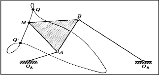
Fig. 2: coupler curve
No attempt is made in path generation to control the orientation of the link that contains the point of interest. The technique of kinematic inversion is also used in path generation.
There are two approaches to synthesis problems graphical & analytical. In our case we go with graphical technique. Though not accurate and precise as the analytical techniques which have the computation assistance from software like MATLAB, MathCad etc to solve the tedious vector equations, but it gives fairly accurate results that is easy to understand, apply and fast to deduce. The graphical synthesis is done on a sheet of paper with
the kinematic dimensions of the links being scaled to some finite proportion.
III. Coupler curves
A four – link mechanism is capable of providing two different types of output motion. These output motion can be derived either from the follower link or the coupler link. The coupler of a four bar linkage may be thought of as a plane extending in all directions but connected to the input and output links through turning pairs. When the linkage is put into motion, any point attached to the plane of the coupler generates some path/curve with respect to frame link, this path is called the coupler curve. It can be easily verified that coupler points, coincident with the pin connections, will generate simple circles with fixed pivots as centres. The other points generally trace much more complex curves.
IV. GRAPHICAL APPROACH
Hrones and Nelson proposed an atlas of approximately 7,300 coupler curves that are drawn to large scale. These atlas constitute a very practical tool to design. One needs to select a segment of suitable coupler curve, in accordance with the required path to be traced by the coupler point, and selecting corresponding linkage and coupler point out of these collections of coupler curves.
The number of coupler curves is infinite. Useful curves can be obtained by choosing proper link proportions and also by selecting suitable locations for coupler point on the floating link. Usefulness of a coupler curve depends on particular shape of its segments and also on a peculiar shape of the curve as whole or part of it. As the interest lies in motion characteristics of the coupler point, the coupler point becomes the output of the linkage.
IJSER © 2013 http://www.ijser.org
International Journal of Scientific & Engineering Research, Volume 4, Issue 7, July-2013
ISSN 2229-5518
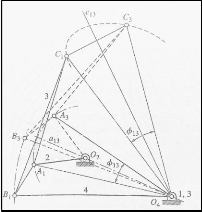
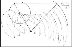
Fig. 3: sample coupler curve form Hrones and
Nelson atlas
2137
To synthesize a linkage so that the coupler will pass through four precision positions, we use point position reduction method and locate any four points C1, C2, C3 and C4 on the desired path (see fig.
4). Choosing C1 and C3 say, we first locate O4
anywhere on the mid normal c13. Then, with O4 as a
centre and any radius R, we construct a circular arc.
Next, with centres at C1 and C3, and any other radius r, we strike arcs to intersect the arc of radius R. These two intersections define points A1 and A3 on the input link. We construct the mid normal a13 to A1A3 and note that it passes through O4. We locate O2 anywhere on a13. This provides an opportunity to choose a convenient length for the input rocker. Now we use O2 as a centre and draw the crank circle through A1 and A3. Points A2 and A4 on this circle are obtained by striking arcs of radius r again about C2 and C4. This completes the first phase of the synthesis; we have located O2 and O4 relative to the desired path and hence defined the distance O2O4. We have also defined the length of the input member and located its positions relative to the four precision points on the path.
Our next task is to locate point B, the point of the attachment of the coupler and output member. Any one of the four locations of B can be used; in this case we use the B1 position. Before beginning the final step, we note that the linkage is now defined. Four arbitrary decisions were made; the location of O4, the radii R and r, and the location of O2. Thus and infinite number of solutions are possible.
Fig. 4: path generation - 1
Referring to fig 4.3. Locate point 2 by making triangles C2A2O4 and C1A12 congruent. Locate point 4 by making C4A1O4 and C1A14 congruent. Points 4, 2 and O4 lie on a circle whose centre is B1. So B1 is found at the intersection of the mid normals of O42 and O44. Note that the procedure used causes points 1 and 3 to coincide with O4. With B1 located, the links can be drawn in place and the mechanism tested to see how well it traces the prescribed path.
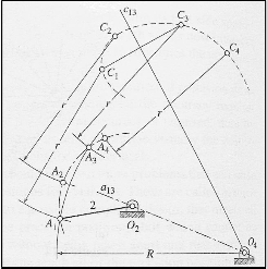
Fig 5: path generation - 2
Referring to fig 6. Locate point 2 by making triangles C2A2O4 and C1A12 congruent. Locate point 4 by making C4A1O4 and C1A14 congruent. Points 4, 2 and O4 lie on a circle whose centre is B1. So B1 is found at the intersection of the mid normals of O42 and O44. Note that the procedure
IJSER © 2013 http://www.ijser.org
International Journal of Scientific & Engineering Research, Volume 4, Issue 7, July-2013
ISSN 2229-5518
2138
used causes points 1 and 3 to coincide with O4. With B1 located, the links can be drawn in place and the mechanism tested to see how well it traces the prescribed path.

Fig. 6: path generation - 3
V. Roberts – Chebychev Theorem
Three different planar, pin jointed four bar linkages
will trace identical coupler curves. This is also described as two different planar slider crank linkages will trace identical coupler curves or the coupler curve of a planar four bar linkage is also described by the joint of a dyad of an appropriate six bar linkage.
When the designer’s concern is only with the curve traced out by a coupler point of a planar four bar, then other planar linkages tracing an identical coupler point may be found by the application of the Roberts – Chebychev theorem.
In the figure below let O1ABO2 be the original four
– bar linkage with a coupler point P attached to AB.
The remaining two linkages defined by Roberts – Chebychev theorem were termed as cognate linkages.
The construction is evident by observing that there are four similar triangles, each containing the angles α, β, and γ and three different parallelograms.
A good way to obtain the dimensions of the two cognate linkages is to imagine that the frame connections O1, O2 and O3 can be unfastened. Then pull O1, O2 and O3 away from each other until a straight line is formed by the crank, coupler and follower of each linkage. If we were to do this for fig. We would obtain fig. Note that the frame distances are incorrect, but all the movable links are of correct length and all the angles are correct.
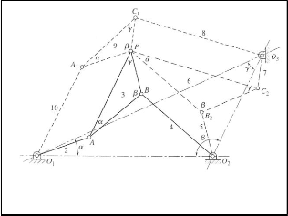
Fig. 7: Roberts – Chebyshev Theorem – 1
The above approach was discovered by A. Cayley and is called Cayley diagram. If the tracing point P is on the straight line AB or its extensions, a figure like fig is of little help because all three linkages are compressed into a single straight line. An example is shown in fig 8 where O1ABO2 is the linkage having a coupler point P on an extension of AB. To find the cognate linkages, locate O1 on an extension of O1O2 in the same ratio as AB is to BP. Then construct in order, the parallelograms O1A1PA, O2B2PB and O3C1PC2.
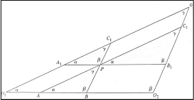
Fig. 8: Roberts – Chebyshev Theorem – 2
IJSER © 2013 http://www.ijser.org
International Journal of Scientific & Engineering Research, Volume 4, Issue 7, July-2013
ISSN 2229-5518
2139
VI. Parallel Motion
It is quite common to want the output link of a mechanism to follow a particular path without any rotation of the link as it moves along the path. Once an appropriate path motion in the form of a coupler curve and its four bar linkage have been found, a cognate of that linkage provides a convenient means to replicate the coupler path motion and provide curvilinear translation (i.e. no rotation) of a new, output link that follows the coupler path. This is termed as parallel motion. Its design is best described by the procedure given below and the same we have utilised to design our linkage.
1. Fig 9 shows the chosen Grashof crank – Rocker four bar linkage and its coupler curve. The first step is to create the Roberts diagram and find its cognates as shown in fig. The Roberts linkage can be found directly, without resorting to cayley diagram, as described earlier. The fixed centre OC is found by drawing a triangle similar to the coupler triangle A1B1P with base OAOB.
2. One of a crank – rocker linkage’s cognates will
also be a crank – rocker and the other is a Grashof double – rocker. Discard the double – rocker, keeping the links numbered 2, 3, 4, 5, 6 and 7 in fig
10. Note that links 2 and 7 are the two cranks and both have the same angular velocity.
3. Draw the line qq parallel to OAOC and through point OB as shown in fig 11.
4. Without allowing links 5, 6 and 7 to rotate, slide them as an assembly along the lines OAOC and qq until the free end of link 7 is at point OA. The free end of link 5 will then be at a point OB and point P on link will be at P .
.
5. Add a new link of length OAOC between P and P . This is the new output link 8 and all points on it describe the original coupler curve as depicted at points P, P
 P
P in fig 11.
6. The mechanism shown in fig 11 has 8 links, 10
revolute joints and one D.O.F. when driven by
either crank 2 or 7 all points on link 8 will duplicate the coupler curve of point P.
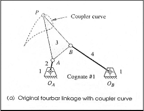
Fig. 9: Parallel motion - 1
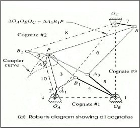
Fig. 10: Parallel motion - 2
IJSER © 2013 http://www.ijser.org
International Journal of Scientific & Engineering Research, Volume 4, Issue 7, July-2013
ISSN 2229-5518
2140
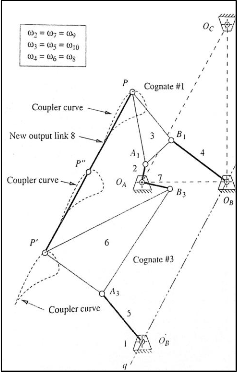
(c) Cognate #3 shifted with OC moving to OA
Fig. 11: Parallel Motion - 3
7. Another common method of obtaining the parallel motion is to duplicate the same linkage (i.e. the identical cognate), connect them with a parallelogram loop and remove the two redundant links. The above technique also results in an eight link mechanism as shown in fig. 12
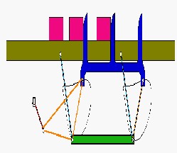
Fig. 12: Parallel Motion generated in a transporter linkage
VII. Model construction
The linkage is modelled and assembled on Solid Edge CAD software and is simulated for prescribed motion characteristics. The final construction yields the model which after rework and fitment undergoes trial run and is found to meet the prescribed motion characteristics.
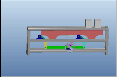
Fig. 12: assembled model front view
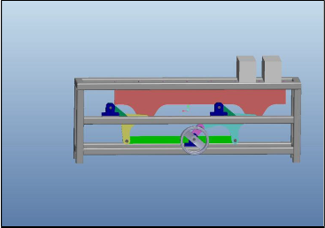
Fig. 13: assembled model back view
IJSER © 2013 http://www.ijser.org
International Journal of Scientific & Engineering Research, Volume 4, Issue 7, July-2013
ISSN 2229-5518
2141
VIII. REFERENCES:
1. Design of Machinery - R.L Norton
2. Mechanisms and Mechanical Devices - Neil
Sclater & Nicholas Chironis
3. Mechanisms & Machines – Amitabha
Ghosh, A.K Mallik
4. Mechanism & Machine Theory – Ashok. G Ambekar
5. Kinematic synthesis of linkages - R.
Hartenberg & J. Denavit
6. Theory of Machines and Mechanisms - Joseph E. Shigley, Gordon Pennock.
7. www.nptel.iitm.ac.in
IJSER © 2013 http://www.ijser.org