International Journal of Scientific & Engineering Research, Volume 4, Issue 12, December-2013 1445

ISSN 2229-5518

Breast Cancer detection System based on Comprehensive Wavelet

Features of Mammogram Images and Neural Network

Sardar P.YabaPhD.

Medical Physics, Physics Department, Education College, University of Salahaddin-Erbil, Iraqi Kurdistan, Iraq

Abstract: The diagnosis system of mammogram images of breast cancer mainly consists of image preprocessing which includes image enhancement and image deionizing feature extraction, and classification. The feature extraction plays a very important role in breast cancer classification system. This paper is presented the comprehensive statistical texture feature extraction method uses Haar DWT. The proposed algorithm calculates max and min medians as well as the standard deviation and average of detail images obtained from wavelet filters, then comes by feature vectors and attempts to classify the given mammogram using a probabilistic neural network with a single hidden layer. In this study along with the proposal of using median of optimum points as the basic feature and its comparison with the rest of the

statistical features in the wavelet field, the relational advantages

guide” with high sensitivity and specificity for detecting of breast cancer [2]. Among all medical imaging techniques that used in cancer diagnosis, digital mammogram is a convenient and easy tool in classifying tumors and many applications in the literature prove their effectiveness in breast cancer diagnosis. Two major of mammographic abnormalities in breast cancer is calcifications and masses. Calcifications are small mineral deposits within the breast tissue, which look like small white
spots on the films. They are often important and

IJSER

of Haar wavelet is investigated. This method has been experimented on a number of malignant and benign mammogram. The experimentation shows that proposed method improves the performance. Amongst the other advantages, high speed and low calculating load are prominent because it’s not involve image segmentation, hence reduce computational complexity.

Index Terms- breast cancer recognition, DWT, classification, neural networks, and statistical features.

I INTRODUCTION

Brest Cancer is the most prevalent cancer among women. It is well known that there is no technology at present, which is capable of curing cancer. But, it is well known that early detection of cancer can aid in good recovery and prolong patient life [1]. The conventional method in medicine screening tool (mammogram) for image classification and tumor detection is by clinician inspection; these methods are often impractical for large amounts of data involved and are also not reproducible. This is especially so for images from women with dense breasts, these would lead to serious inaccuracies classification. Thus, there is a need for more effective methods. According to Dio et al., the purpose of Computer-Aided Diagnosis (CAD) in radiology, is “to improve the diagnostic accuracy as well as the consistency of radiologists’ image interpretation by using the computer output as a
common findings on a mammogram. They can be
produced from necrotic cellular debris or from cell
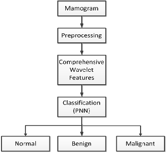
secretion.[3]. Calcifications can appear with or without an associated lesion, and their morphologies and distribution provide clues as to their etiology as well as whether they can be associated with a benign or malignant process. The classification pipeline used in this work is shown in Figure 1. Though CAD systems are thought to be in a nascent stage, evidence in [4] proves quite the contrary with high success rates for radiologists using CAD systems.

International Journal of Scientific & Engineering Research, Volume 4, Issue 12, December-2013 1446

ISSN 2229-5518

2. OVERVIEW OF PROPOSED APPROACH

In this paper, the tumor can be detected by using comprehensive wavelet statistical features, derived from all subbands of decomposition. The following is the presentation of major stages of computation used to classify digital mammograms:

Figure 1: Classification stages for proposed system.

There are numerous works which have been done in the past with a Wavelet transform is capable of

2.1. PREPROCESSING

The aim of preprocessing is to improve the
image data by suppressing the undesired distortions or enhances some image features relevant for further processing and analysis task. Figure 2 shows the flow diagram for the steps employed in preprocessing stage. In order to reduce the memory requirement of the device and considering the breast topography, the test images have been cropped to emphasize the breast tissue to a size determine by the Matlab function imcrop:
[I1,Dim]=imcrop(I)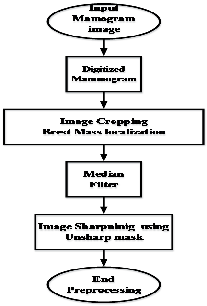

providing the time and frequency information
simultaneously. Especially, the width of the window is changed as the transform is computed for every single spectral component, which is probably the most significant feature of the wavelet transform. Wavelet analysis generates an estimate of the local frequency content of a signal by representing the data using a family of wavelet functions that vary in scale and position. By using wavelet analysis, we can identify locally periodic trends in the signal. [5]
This paper proposes a system designed to perform prescreening of digital mammograms for the presence of microcalcifications based on wavelet decomposition statistical measurements collecting its information from all subbands in different levels of decomposition . In this study a
viable algorithm with high precision and low calculating load was proposed to classify malignant and benign mammogram images using wavelet transform and its combination with statistical features of resulted images and using a probabilistic neural network (PNN). Second part involves a review of wavelet transform and proposed algorithm for features deduction. The result appears in part three and finally part five concludes the article.
Figure 2 preprocessing
Dim in the previous code represents the
(x,y)coordinates of the four corners of the new window. A median filter is employed (nonlinear filter) which is an efficient tool in removing salt and pepper noise, median tends to keep the sharpness of image edges while removing noise the size of the window used is [3 3] the Matlab code for median filter used in proposed system is shown below.

D=medfilt2 (I,[3 3]);

International Journal of Scientific & Engineering Research, Volume 4, Issue 12, December-2013 1447

ISSN 2229-5518

The denoised image D still has low intensity contrast and may have non uniform brightness caused by the position of light sources. The unsharp
The standard DWT is implemented with the help of appropriately designed Quadrature Mirror filters (QMF). It consists of low-pass coefficients
mask algorithm has been used for denoised image
sharpening. These two steps (denoising and

g[n]

and high-pass coefficients

h[n]

enhancement) used to obtain well distributed texture image which suit very effective for feature
where n = 0 ⋅ ⋅ ⋅ L . These two impulse responses thus
related with the scaling and wavelet functions as:
extraction.

4. FEATURE EXTRACTION

φ ( x) =
ψ ( x) =

2 ⋅ ∑ g[n] ⋅ φ (2 x − n)

n∈Z

2 ⋅ ∑ h[n] ⋅ φ (2 x − n)

n∈Z

(2)
(3)
The purpose of feature extraction is to
reduce the original data set by measuring
certain properties, or features, that distinguish
The products of above 1-D wavelet and scaling functions can be used to obtain the 2-D
scaling and wavelet functions from (4)-(12).
one input pattern from another. The extracted
features provide the characteristics of the input type to the classifier by considering the description of the relevant properties of the image [6].Statistic features such as mean, variance, and standard deviation in transform domain using
φ (i, j) = φ (i) ⋅ φ ( j) ψ 1 (i, j) = φ (i) ⋅ψ ( j) ψ 2 (i, j) = ψ (i) ⋅ φ ( j) ψ 3 (i, j) = ψ (i) ⋅ψ ( j)
(4) (5) (6)
(7)
Wavelet are extracted from the detected
Equation (4) known as approximation

IJSER

microcalcifications images.

Discrete Wavelet Transform (DWT):

In a kind of wavelet transform used in this study, the transform uses two filter sets of high
pass and low pass and applies them on the given signal (image) in some layers. As the image crosses
theses filters for the first time, four new images are acquired; approximation (result of the low pass
filter), details in horizontal point, details in vertical point, and details in diameter. In order to calculate
wavelet coefficients in two layers (scales), for second time the approximated image from previous
stage should be transmitted from those filters. This process can be also repeated for the rest of scales.
In each wavelet transform application, the dimensions of resulted image cut into two halves.
Thus the DWT decomposes an image

f (x, y ) ∈ L2 (R 2 ) into the form of set of dilation and

coefficients (cA) and the remaining three are known as detail coefficients (cH, cV, cD). The cH, cV, and cD sub-bands give the information in horizontal, vertical, and diagonal direction. Thus, the filters divide the input image into aforementioned four non-overlapping multi- resolution sub-bands cA, cH, cV, and cD. The sub- band cA represents coarse-scale DWT coefficients while the sub-bands cH, cV, and cD represent the fine scale DWT coefficients. In order to obtain the next coarser scale of wavelet coefficients, the sub- bands cA is further decomposed to get again the four sub-bands as shown in Figure .3.
translation of wavelet functions scaling function φ ( x, y) [7].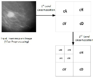

ψ l (x, y ) and

f ( x, y) = ∑k∈Z 2 s j 0, k ⋅ φ j 0, k ( x, y) + ∑ ∑ ∑ wj , k ⋅ψ j , k ( x, y)

l l

l∈θ j ≥ j 0k∈z 2

j 0 j 0

(1)
Where φ j 0,k ( x, y) = 2
⋅ φ (2
( x, y) − k ) ,
ψ l ( x, y) = 2 j
⋅ψ (2
j ( x, y) − k )

IJSER © 2 http://www.ijser.org

International Journal of Scientific & Engineering Research, Volume 4, Issue 12, December-2013 1448

ISSN 2229-5518

Figure .3 Sub-band decomposition

V. FEATURE VECTOR

After preprocessing of mammogram images, wavelet transform filters were applied on the each image to deduct vector of image features.
Thus, each mammogram image is decomposed up to two level. For the first level of decomposition three details matrices (image) were obtained in three different points as well as an approximation matrix. Wavelet transform of an image, measures light fluctuation in different Scales. Wavelet coefficients in edges of image structures turn max because of improvement in
feature which is equal 1 for normal breast and 2 for cancer breast images).

Classification

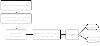
The task of classification plays an important role for domain practitioners using medical images. The classification process involves grouping objects into pre-defined classes or finding the class to which an object belongs. Figure4 contains an illustration of proposed classification scheme.

Output of Preprocessing

Statistical feature Extracted from Haar Wavelet

local contrast. Therefore, max points of details coefficients can be used as an index for probable errors [8]. To avoid segmentation of the image and

Normalized

Feature vector

Generation of Training and

Testing data

PNN

Malignant

Benign

to decrease calculation load, median of max points
was calculated. Also to increase sensitivity and precision, median of each image min was

Figure 4: Classification process

Databank

IJSER

calculated along with Energy and standard
deviation of approximation matrix as well as the
Energy and standard deviation of details matrices then was added to image features. The energy and standard deviation for each sub-band are computed as the texture feature vector using equations (8) and (9) respectively.
1 M N
In this work, the mammograms obtained from the Mammographic Image Analysis Society (MIAS) Mini Mammographic database are used to test the proposed algorithm. The use of such a database aids in comparison of CAD algorithms through evaluation using a common database. The texture feature was extracted from 50 mammogram.
25 for normal patients and 25 for cancer patients.

Ek =

N ∑ ∑ ck (i, j)

× i =1

j =1

(8)

Generating Training and Test Data

σ k =

M × N

∑

i =1

∑ (ck

j =1

(i, j) − µ k

(i, j))
(9)
In order for MATLAB to perform the analysis, the data are arranged in an alternative
sequence in a table , training file is created for
Where Ek and

σ K are the energy and

familiarizing with the data and its classes. A total

standard deviation for the kth sub-band of dimension M × N with coefficients ck (i, j).

Hence, at each scale, energy and standard deviation based features are computed and the resultant feature vector is given by (10) fv=[median_max_details median_min_details E(cA) Std(cA) Std(cH) Std(cV) Std(cD) S(cA1) E(cA1) E(cV1) E(cD1) E(cH1) class]

(10)
The above feature vector is calculated for
each image sample (malignant and benign) and stored as feature vector, then every feature value for every sample is normalized (except the class
of three training data are created: training 1,
training 2 and training 3. Traning1 was generated
from the first 16 data taken from the alternative class consisting of normal and breast cancer patients in sequence . Training 2 is done in a similar method but the data is selected from the middle portion consisting 16 of the normal and cancer breast, while training 3 consists of data from the bottom last 16 data. Testing files are created and input into a classifier for classification according to its accuracy and sensitivity from the normal and cancer breast classes.

International Journal of Scientific & Engineering Research, Volume 4, Issue 12, December-2013 1449

ISSN 2229-5518

A total of three testing data are created:
1 ni

 − (x − x(i ) )t (x − x(i ) )

testing 1, testing 2 and testing 3. Testing1 is

p(x | s ) = ( )

∑exp j j 
created from the last 32 data from the normal and cancer breast images respectively. Testing 2 is

i 2π

m / 2 m i

| si | j=1 
2σ 2
 (11)
done in a similar method but the data is selected
where

p(x | si )

is the probability of vector x
from the first and last 32 of the normal and cancer
occurring in set si, corresponding to the type of
(i )
breast data, while testing 3 consists of data from the
fault;
x j =jth exemplar pattern or training pattern
first 32 data.
Probabilistic neural network
The most important advantage of PNN is the simple structure, training manner and only one free parameter, the smoothing factor, which have to be adjusted by the user and this factor can be adjusted at run time without the requirement of network retraining. Probabilistic Neural Network has been used for the purpose of classification
belonging to class si, type of fault; ni is the cardinality of the set of patterns in class si ; m is total number of training patterns; σi is smoothing parameter.
The summation layer is used to compute the sum from the previous layer:

pr (si | x) = p(x | si )pr (si )

p(x) (12)

Where pr (si | x) , i=1,2,…..k is the priori PDF

because of its high versatility and accuracy as
compared to back propagation.
of the pattern in classes to be separated;

pr (si ) is

The PNN has three layers. When an input is presented, the first layer computes distances from
priori probabilities of the classes;
to be constant.

p(x)

is assumed

IJSER

the input vector to the training input vectors, and
The decision rule is to select class Si of the
produces a vector whose elements indicate how
fault type, for which

pr (Si | x) is maximum.

close the input is to a training input. The second
layer sums these contributions for each class of inputs to produce a vector of probabilities as its net output. Finally, compete transfer function on the output of the second layer picks the maximum of these probabilities, and produces a 1 for that class and 0 for the other classes.
The input layer is fully connected to the hidden layer. Feature vectors are normalized and used as inputs of this network. The hidden layer has a node for each classification. Each hidden node calculates the dot product of the input vector with a test vector subtracts 1 from it and divides the result by the standard deviation squared. Also the input node corresponds to the mean wavelet coefficient for both of classes – benign and malignant. The outputs correspond to the two classes benign and malignant. A winner – take – all decision rule (largest output wins) gave the expected classification.
The activation function of a neuron, in the
case of the PNN, is statistically derived from estimates of probability density functions (PDFs) based on training parameters (Bose and Liang,
1998). Estimator for the PDF is:
The variable σ is a smoothing factor that, in
effect, determines the Gaussian window width. For
the two–dimensional input case, a small value of σ gives distinct modes corresponding to the locations of training samples [9]. As the value of σ increases, the degree of interpolation also increases. A universal smoothing factor (σ = 0.5) was selected using the criterion of percent classification of the smoothing dataset.
VII. EXPERIMENTAL RESULTS
The proposed method is tested by using the
mini- MIAS database of mammograms. All images are digitized at the resolution of 1024 × 1024 pixels and 8-bit accuracy (gray level). The texture feature was extracted from 50 mammogram. 25 for normal patients and 25 for cancer patients.
The original image is shown as Fig.4 (a).
The preprocessing is done by cropping, and denoising using median filter and contrast enhancement which are shown in Fig.4 (b), (c), (d) respectively.

International Journal of Scientific & Engineering Research, Volume 4, Issue 12, December-2013 1450

ISSN 2229-5518

wavelet has been applied.

(a) (b)

(c) (d)
Figure 5: Preprocessing output
Figure 6: 2-level Haar Wavelet decomposition.

IJSETo stuRdy the data distribution of the features

After preprocessing of the mammogram image samples, the samples are introduced to
2-level Haar wavelet decomposition wavelet which
is prominent in terms of memory consumption and despite other wavelets, without any influence of edge, is completely recursive. Haar wavelet does not possess overlap windows and only reflects the changes between two adjacent pixels [2]. Also since it uses just two scales and wavelet, it calculates average and difference of a pair. The subbands decomposition for the above image is shown below in figure 6. Which is shows digital mammogram image (malignant image) along with approximation images and horizontal, vertical, and diameter details after wavelet transform in a scale
extracted by the proposed diagnoses system, the
features were plotted as their empirical Cumulative Distributive which is seen in Figure 3. This visualization technique helps in better inference of variations in feature spread obtained using DWT despite other wavelets, without any influence of edge, is completely recursive.
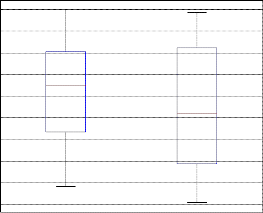
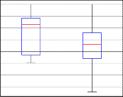
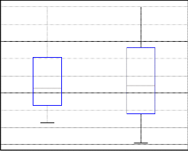
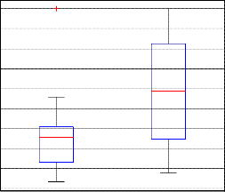
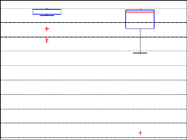
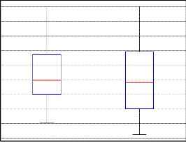
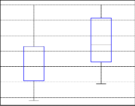
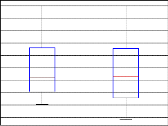
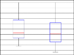
All the levels of sub-bands of DWT was used to extract the features. To study the data distribution of the features extracted by DWT, the 12-extracted features were plotted as box plot in Figure 7 in which each graph contains two boxes first has been calculated from the malignant images while the other calculated from benign images. This
visualization technique helps in better inference of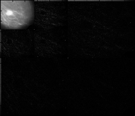

with

100

150

200

Decomposition at level 2

Haar
variations in feature spread obtained using DWT. Feature ranking or selection was not performed due to the fact that it is quite evident that all sub-bands of a wavelet transformation scheme are important as information missing in one sub-band is always found in another.

250

300

350

400

450

500

50 100 150 200 250 300 350 400 450 500

International Journal of Scientific & Engineering Research, Volume 4, Issue 12, December-2013 1451

ISSN 2229-5518

0.9

0.8

0.7

0.6

0.5

0.4

0.3

0.2

0.1

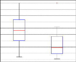
Benign Malignant median max(cH,cV,cD)

0.9

0.8

IJSE0.6 R

0.5

0.4

0.3

0.2

0.1

Benign Malignant median min(cH,cV,cD)

0.9

0.8

0.7

0.6

0.5

0.4

0.3

Benign Malignant standard Deviation(cA)LL

Figure 7: Continue

International Journal of Scientific & Engineering Research, Volume 4, Issue 12, December-2013 1452

ISSN 2229-5518

0.95

0.9

0.85

0.8

0.75

0.7

0.65

0.9

0.8

0.7

0.6

0.5

0.4

0.3

0.6

0.55

Benign Malignant standard Deviation(cA)LL

0.2

Benign Malignant standard Deviation(cD)

1 1

0.9

0.95

0.8

0.7

0.6

0.5

0.4

0.3

0.2

0.9

0.85

0.8

0.75

0.7

0.65

0.6

0.55

0.1

Benign Malignant standard Deviation(cH)

Benign Malignant standard Deviation(cA1)LL1

0.9

0.8

0.7

0.6

0.5

0.4

0.9

0.8

0.7

0.6

0.3

0.2

0.1

Benign Malignant standard Deviation(cV)

0.5

0.4

Benign Malignant

Energy (cA1)LL1

Figure 7: Continue

International Journal of Scientific & Engineering Research, Volume 4, Issue 12, December-2013 1453

ISSN 2229-5518

0.9

0.8

0.7

0.6

0.5

0.4

0.3

0.2

into this network. To assess the result of proposed diagnosis system, two criteria of accuracy, and specificity, defined in table 1 were used.
TABLE I
PERFORMANCE EVALUATION CRITERIA

0.1

0.9

0.8

Benign Malignant

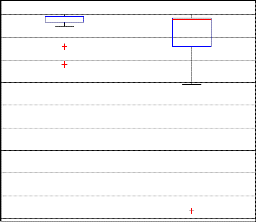
Energy (cD1)

While, TP is the rate of true positive, TN is the rate of true negative, FP is the rate of false positive, and FN is the rate of false negative [10]. Achieving high specificity means that few cases unnecessary recommended for cancer detection. While a high sensitivity means that few cancers will be missed. The most important parameter is sensitivity since errors in recognizing cancerous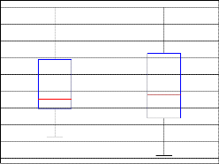

lesions are life-threatening. Errors in recognizing

0.7

0.6

0.5

0.4

0.3

0.2

0.1

TN’s are not life-threatening but they do cause stress and anxiety and waste of resources and may be money [8]. The performance of proposed diagnosis system detection is compared with the results presented in [11] (also wavelet had been used to extract features for breast cancer images). The result is shown below in table 2

Benign Malignant

0.9

0.8

0.7

0.6

0.5

0.4

0.3

0.2

0.1

Energy (cH1)

Benign Malignant

Energy (cV1)

Table 2 results of Classifier

Classifiers	Sensitivity	Specificity
Propose Scheme	100%	66.66%
Algorithm in[11 ]	90%	80%

The proposed diagnosis system outperform the system presented in [11] by 10% in sensitivity which is the dominant factor in any CAD system.
VIII. CONCLUSION
The proposed method divides the image into eight sub-images using Haar wavelet and derives the local features separately from each region. The experimental analysis illustrates that suggested

Figure 7: The proposed Comprehensive 12-feature plot for

malignant and benign breast images samples

Finally a probabilistic neural network was used for classification and features vector was fed
method increase the sensitivity by 10% as compared with the algorithm presented in [11]. It is also observed that proposed method reduce the complexity of calculation because it avoid

International Journal of Scientific & Engineering Research, Volume 4, Issue 12, December-2013 1454

ISSN 2229-5518

segmentation of the image and to decrease calculation load, median of max points was calculated. Also to increase sensitivity. Finally Simulations in the MATLAB showed excellent results

IX. REFERENCES

[1]. Heang-Ping C, Sahiner B, Helvie MA, Petrick N, Roubidoux MA, Wilson TE, Adler DD, Paramagul C, Newman JS & Sanjay-Gopal, S. Improvement of radiologists’ characterization of mammographic masses by using computer-aided diagnosis: an ROC study. Radiology 212, 817-827 (1999).

[2]. Karthikeyan Ganesan, et al” Automated Diagnosis of Mammogram

Images of Breast Cancer Using Discrete Wavelet Transform and Spherical Wavelet Transform Features: A Comparative Study” , An Open Access Journal, ISSN 2326-0912 Published June 5, 2013

Adenine Press (2013)

[3]. Doi K, MacMahon H, Katsuragawa S, Nishikawa RM & Jiang, Y.

Computer-aided diagnosis in radiology: potential and pitfalls.

European Journal of Radiology 31, 97-109 (1999). DOI: 10.1016/ S0720-048X(99)00016-9.

[4]. Fenton JJ, Taplin SH, Carney PA, Abraham L, Sickles EA, D’Orsi

C, Berns EA, Cutter G, Hendrick RE, Barlow WE & Elmore JG. Influence of computer-aided detection on performance of screening mammography. N Engl J Med 356, 1399-1409 (2007)

[5]. Tsvetelina D. Draganova et al, ” Wavelet based approach for

Fusarium corn kernels recognition using spectral data processing”

10th IFAC Workshop on Programmable Devices and Embedded

Systems 2010

[6]. Essam A. Rashed et al “Neural networks approach for mammography diagnosis using wavelets features”, first Canadian

conference on biomedical computing, 2006

[7]. Amol D. Rahulkar and Raghunath S. Holambe,”Rotation Invariant

Iris TextureVerification”, AKGEC Journal of Technology, vol. 1, pp

1-6 , Jan. 2010 (ISSN-0975-9514).

[8]. M.Ghazvini, S. A. Monadjemi, N. Movahhedinia, and K. Jamshidi

,“Defect Detection of Tiles Using 2D-Wavelet Transform and

Statistical Features”, World Academy of Science, Engineering and

Technology 25 2009

[9]. Specht, D. F. “Probabilistic neural networks and general regression

neural networks”. Fuzzy Logic and Neural network Handbook, ed. C.H. Chen, ch. 3. New York: McGraw–Hill, Inc. 1996

[10]. H. D. Cheng, X. Cai, X. Chen, L. Hu, and X. Lou, “Computer-aided

detection and classification of microcalcifications in mammograms: a survey,” Pat. Rec., vol. 36, pp. 2967-2991, 2003.

[11]. Bibin Binu Simon,Vinu Thomas,Jagadeesh Kumar P” Algorithm for

the Detection of Microcalcification in Mammogram on an Embedded Platform”, International Journal of Scientific & Engineering Research, Volume 4, Issue 4, April-2013