International Journal of Scientific & Engineering Research, Volume 3, Issue 11, November-2012 1
ISSN 2229-5518
Bianchi Type-III String Cosmological Models in The Presence of Magnetic Field in General Relativity
Kandalkar S.P.1, Samdurkar S.W.2 and Gawande S.P.3
1Department of Mathematics, Govt. Vidarbha Institute of Science & Humanities, Amravati (India).
1 spkandalkar2004@yahoo.com,2 seema_samdu@yahho.co.in.3 sskandalkar2010@yahoo.co.in
Abstract— In this paper we have examined Bianchi type-III string cosmological model in the presence of magnetic field. To get determinate solutions, the Einstein’s field equations have been solved for two cases (i) Reddy string and (ii) Nambu string. The physical and geometrical behaviour of these models are discussed.
Index Terms— Bianchi type-III model, Reddy string, Nambu string, Magnetized
.
At very early stage of evolution of universe, it is assumed that during the phase transition, the symmetry of universe is bro- ken spontaneously. It can give rise to topological stable defects such as domain walls, strings and monopoles (Kibble1976).Of all these cosmological structures, cosmic string play a vital role in structure formation in cosmology (Zel’dovich1990).It is believed that the vacuum strings give rise to density fluctua- tions sufficient in formation of galaxies (Zel’dovich1990).The cosmic strings have their stress-energy coupled to the gravita- tional field. Therefore, the study of gravitational effects of such strings will be of interest.
expansion. Therefore considering the presence of magnetic field in strings universe is not unrealistic and has been inves- tigated by many authors (Banerjee et al. 1990;Shri Ram and Singh1995; Singh and Singh1999; Baliand Upadha- ya2003).Banerjee et al.(1990) investigated some cosmological solutions of massive strings for Bianchi type I space time in the presences and absence of magnetic field. Tikekar and Patel (1992) obtained some exact solutions of massive string of Bian- chi type III space time presence and absence of magnetic field. Recently Upadhaya and Dave (2008) have investigated Bianchi type III massive string cosmological model in the presence and absence of magnetic field, under the assumption that the ex-
The present day configuration of the universe is not contra-
pansion
( )
in the model is proportional to the shear
n
( )
dicted by large scale network of strings in the early universe.
The general relativistic formation of cosmic strings, are given
which lead C A
n 1.
and have obtained particular solution for
by Letelier (1979 1983) and Stachel (1980).In string theory, the myriad of particle type is replaced by single fundamental building block, a string. These strings can be closed, like a loop or open, like a hair. As the string moves through time it tress out a tube or a sheet, according whether it is close or open. Since strings are not observed at present time of evolution of universe one can illuminate strings and end up with cloud of particles.
String cosmological models have been studied by many au-
In this paper we have investigated Bianchi type III cosmologi- cal model in the presence and absence of magnetic field. To obtained exact solution field equations, we have considered Reddy string and Nambu string. The physical behaviour of models are also discussed.
We consider the Bianchi type III space time in the form
thors. A number of general relativistic exact solution were in- vestigated for Bianchi type II,VI0 ,VIII & IX string cosmologi-
ds 2 dt 2 A2 dx 2 B 2 e2x dy 2 C 2 dz 2
(1)
cal models by Krori et al.(1990). A class of cosmological solu- tions of massive strings for Bianchi type VI0 space time has been obtained by Chakraborty (1991). Roy and Banerjee (1995) have investigated some LRS Bianchi type II string cosmologi-
where A, B and C are functions of t only and is a constant.
The energy momentum tensor for a cloud of string dust with magnetic field along the z-direction of the string is given by
cal models which representgeometrical and massive strings. Wang (2004 2005 2006) has investigated and discussed some
Tij
uiu j
xi x j
1
lm
Fil Fjm
1
gij Flm F
lm
(2)
cosmological models and their physical implication in some
Bianchi type space times.
The magnetic field has important role at the cosmological scale
4 4
where ui and xi satisfy the conditions
and is present in galactic and intergalactic spaces. The im-
ui u
xi x
1
u i x 0
(3)
portance of the magnetic field for various astrophysical phe-
nomenon has been studied in many papers. Melvin (1975) has
is the energy density for a cloud string with particles at-
pointed out that during the evolution of universe, the matter is
tached to them, is the string tension density,
u i is the four-
in highly ionized state and is smoothly coupled with the field,
subsequently forming neutral matter as a result of universe
velocity of the particles, and xi is a unit space-like vector rep-
IJSER © 2012
International Journal of Scientific & Engineering Research, Volume 3, Issue 11, November-2012 2
ISSN 2229-5518
resenting the direction of string. In a co-moving coordinate system, we have
with four unknown parameters , , A and C .One addition- al constraint relating these parameter is required to obtain
u i (0,0,0,1) ,
![]()
x i (0,0, 1 ,0) , (4)
C
explicit solutions of the system. We assume that the expansion
( ) is proportional to the shear ( ). This condition lead to
The particle density of the configuration is given by
p
(5)
C An
where n is a constant.
(16)
The electromagnetic field tensor
Fij
has only the non-zero
To obtain exact solutions, we solve the field equations for the
component
F12 because the magnetic field is assumed to be
following two cases.
along the 𝑧-direction. Subsequently Maxwell equation
Fij ,k Fjk ,i Fki , j 0
and
F ij
( g )
![]()
12 0
;k
In this case
0
From (13), (14) and (17) we obtain
(17)
lead to
A C
A 2
A 2 K 2
F12
Ke x
(6)![]()
![]()
AC A2
![]()
![]()
![]()
0
A A2 A4
(18)
where K is a constant so the magnetic field depends upon the space
Using (16), the above equation reduces to
coordinate x only. From (2), (4) and (6), it follows that F14 0 .
A
A 2
2 K 2
The Einstein’s field equation
1
![]()
![]()
(n 1)
A A2
![]()
![]()
A2 A4
(19)
Rij
![]()
Rg ij 8Tij
2
(7)
Let A
f ( A) which impliesthat A
ff , where
for the metric (1) lead to the following system of equations:![]()
f df .
A B BC A C K
8
dA
(8)![]()
![]()
![]()
![]()
AB BC
![]()
AC A2 A4
Hence (19) can be written as
2 2
B
![]()
B
![]()
C
C
![]()
![]()
BC K 0
BC A4
(9)![]()
![]()
d f 2 2(n 1)
dA A
![]()
f 2 2
A
![]()
2 K A3
(20)
By integrating (20) we find
A
![]()
A
![]()
C
C
![]()
![]()
A C K 0
AC A4
(10)![]()
f 2
![]()
K A2 MA2( n1)
(21)
n 1 n
2 2
![]()
![]()
![]()
![]()
![]()
A B A B K
8
(11)
where M is integration constant. Therefore, we have
A B AB A2 A4
dA 2 K 2
A2 MA2( n1)
![]()
A
B
![]()
dt
![]()
n 1 n
![]()
![]()
0
A B
(12)
(22)
Thus the metric (1) reduces to the form
where a dot (.) over a variable denotes ordinary differentiation with
dt
respect to time t. From equation (12), we have two cases 0 and![]()
ds 2
dA2 A2 dx 2 A2 e 2x dy 2
A B .When 0, the metric (1) degenerates into Bianchi type
I. Since we have considered Bianchi III symmetry, we assume that
is non-zero and A B . Thus the field equations (8)-(11) reduces
as
dA
A2 n dz 2
dT 2
![]()
T 2 dx 2
(23)
2 A C A K
8
(13)![]()
![]()
K
A2
MA
2( n1)
(24)![]()
![]()
![]()
![]()
AC A2 A2
2 A A K
A4
2
8
(14)
n 1 n
T 2 e 2x dy 2 T 2 n dz 2
![]()
![]()
![]()
A A
A2
C
![]()
A2 A4
A C K 2
where A T , x X , y Y , z Z
In the absence of magnetic field i.e. when K 0 then![]()
![]()
![]()
![]()
0
A C AC A4
(15)
the metric (24) reduces to the form
The field equations (13) -(15) are a system of three equations
IJSER © 2012
International Journal of Scientific & Engineering Research, Volume 3, Issue 11, November-2012 3
ISSN 2229-5518
ds 2
dT 2
T 2 dx 2

1 n(n 1)M
![]()
2 2T 2( n1) n 4
![]()
n 1
![]()
![]()
MA2( n1)
(25)
q 0 if
(n 1) K 2
1
M 3 3
(34)
T 2 e 2x dy 2 T 2 n dz 2
![]()
![]()
2 nT 2
![]()
2( n1)
The energy condition 0 implies that
(n 1)K 2
![]()
nT 2
![]()
(2n 1)M T 2( n1)
n 2
![]()
n 1
(35)
The energy density ( ) , the string tension ( ) , the particle
The particle density
( p
) and tension density
( )
of the
density ( p ) , the scalar of expansion ( ) and the shear ( )
for the model (24) are given by
cloud string vanish asymptotically in general if (n 2) 0
.The expansion in the model stops when n 2 .The model
1
n 2
(n 1)K
(2n 1)M
(26)
starts expanding with a big bang at T 0 and the expansion![]()
![]()
8 (n 1)T 2
![]()
nT 4
![]()
2( n 2)
in the model decreases as time increases if (n 2) 0 .The
1 n 2
(n 1)K 2
(2n
1)M
model (24) has singularity at T 0 .The physical parameters![]()
![]()
![]()
![]()
2( n 2)
(27)
, , p
are infinite at the singularity T 0 and decreases as
8 (n 1)T
2
nT T
2
T .The energy density and expansion in the model de-
1
2n
2(n 1)K
2(2n 1)M
(28)
creases rapidly in the presence of magnetic field. Since![]()
![]()
p 8 (n 1)T 2
![]()
nT 4
![]()
2( n 2)
![]()
1
![]()
lim 0. Hence the model does not approach isotropy for
T
(n 2)
2
K M
(29)
large value of T .For the condition![]()
(n 1)T 2
![]()
![]()
nT 4
2( n2)

1 n(n 1)M
(n 1) 2 2
K 2 M
2T 2( n 1) n 4
2
![]()
![]()
![]()
n K
![]()
![]()
,the solution gives
M
3 (n 1)T 2 nT 4 T 2( n2)
(30)![]()
1 (
![]()
![]()
1) 3 3
2
2 2
nT 2
2( n1)
![]()
![]()
(n 1)
2 3(n 2) 2
const
(31)
accelerating model of the universe and for the condition
n(n 1)M
The deceleration parameter is given by
1
2T 2( n1)
n 4
q
![]()
R / R
![]()
![]()
![]()
(n 1) K 2 M 3 3
R 2 / R 2
![]()
1 2
![]()
nT 2
![]()
2( n1)
, our solution repre-
sents decelerating model of the universe and q approaches at
K 2
M (n 1) 2 2
![]()

4 2( n 2)
2K
![]()
value -1 when![]()
(n 2)M
![]()
.Further under the
![]()
1 n nT T
(32)
nT 2
T 2( n1)
n 1
n 2
2
K 2 M
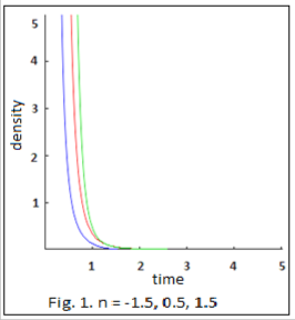
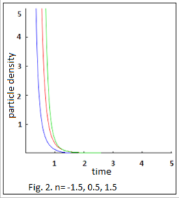
constraint 1, K
1 and M 1, the energy density ( )

![]()
![]()
(n 2)
(n 1)T 2 nT 4 T 2( n 2)
From the (32), we observe that
1 n(n 1)M
and particle density ( p )
n 0 (Fig.1 and Fig.2).
is positive for 2 n 1 and
q 0 if
2T 2( n1)
![]()
![]()
n 4
(33)
1 (n
1) K 2 M 3 3
and![]()
2 nT 2
![]()
![]()
2( n1)
IJSER © 2012
International Journal of Scientific & Engineering Research, Volume 3, Issue 11, November-2012 4
ISSN 2229-5518
(n 2)
2
![]()
1
M
(40)![]()
(n 1)T 2
![]()
2( n2)
2 (n 1) M
(41)![]()
![]()
![]()
3 (n 1)T 2 T 2( n 2)
![]()
![]()
(n 1)
const
(42)
2 3(n 2) 2
In the absence of magnetic field, the particle density ( p ) and tension density ( ) vanish when T .The expansion in the model decreases as time increases if n 2 0 except n 1.![]()
Since lim
T
0 .Then the model does not approach isotropy
for large values of T . Further under the constraint
1, K 1 and M 1, the energy density ( ) and particle
1
In the absence of magnetic field, the energy condition 0
lead to![]()
density ( p ) is positive for 2 n 1 and n .
2
(2n 1)M
![]()
T 2( n1)
n 2
![]()
n 1
(36)
and the physical parameters , , p , and are given
2
1
n
(2n 1)M
(37)![]()
![]()
8 (n 1)T 2
![]()
2( n 2)
1
n 2
(2n
1)M
(38)![]()
![]()
8 (n 1)T 2
2
![]()
2( n 2)
1
2n
2(2n 1)M
(39)![]()
![]()
p 8 (n 1)T 2
![]()
2( n 2)
IJSER © 2012
International Journal of Scientific & Engineering Research, Volume 3, Issue 11, November-2012 5
ISSN 2229-5518
3.2 Case II: Nambu String
![]()
![]()
1
2 3
const
(55)
In this case
The deceleration parameter is given by
From (13), (14) and (43) we obtain
(43)
q
![]()
R R
![]()
1 4n
(56)
R 2 R2
n 2
![]()
![]()
A A C 0
(44)
From (56), we observe that
A AC 1
Using (16), the above equation reduces to
2
![]()
q 0 if n
4
(57)
A
A
and![]()
![]()
n 0
A A
(45)
q 0 if n 1
(58)![]()
4
which on integration gives![]()
![]()
1 1
A (1 n) 1n (at b) 1n
(46)
The energy condition 0 implies that
where a and b are constants of integration.
(2n 1)a2 2 K 2
![]()
![]()
![]()
(59)
Hence we obtain![]()
![]()
1 1
(1 n)2
2 2
(1 n) 1n T 1n
4 4
(1 n) 1n T 1n
B (1 n) 1n (at b) 1n
(47)
The energy density and string tension are infinite at singularity![]()
![]()
n n T 0 and decreasing as
T .The expansion in the model
C (1 n) 1n (at b) 1n
Thus the metric (1) reduces to the form
(48)
stops when n 2 .The model starts expanding with a big bang at
T 0 and the expansion in the model decreases as time increases
![]()
2
ds2 dt 2 (1 n) 1n
![]()
2
(at b) 1 n
dx2
![]()
.Since lim 0 .Hence the model does not approach isotropy for![]()
![]()
2 2 T
(1 n) 1 n (at b) 1 n e2x dy2
![]()
![]()
2n 2n
(1 n) 1n (at b) 1n dz 2
(49)
large value of T .The model (50) has singularity at T 0 . For the
1
After a suitable transformation of coordinate, the metric (49)
takes the form
condition![]()
n the solution gives accelerating model of the uni-
4
1
ds 2
![]()
dT 2
![]()
2
(1 n) 1n T
![]()
2
1n dX 2
verse and for the condition n ![]()
, ours solution represents deceler-
4
a 2
2 2 x n n
ating model of the universe and q approaches at value -1 when
(1 n) 1n T
1n e 2
![]()
![]()
![]()
![]()
2 2
dY 2 (1 n) 1n T 1n dZ 2
(50)
n 1 .Further under the constraint 1 and K 1, the energy
where T ax b, x X , y Y , z Z
The energy density ( ) , the string tension ( ) , the particle density
( p ) , the scalar of expansion ( ) and the shear ( ) for the mod- el (50) are given by
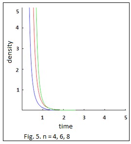
density is positive for n 4 (Fig.5).
1 (2n 1)a 2 2
![]()
![]()
![]()
K 2
![]()
p 0
8 (1 n) T
2
(1 n) 1n T
2
1n
4
(1 n) 1n T
(51) (52)
1n
![]()
a(n 2) (1 n)T
2
(53)
2
(n 2)a
![]()
3(1 n)2 T 2
(54)
IJSER © 2012
International Journal of Scientific & Engineering Research, Volume 3, Issue 11, November-2012 6
ISSN 2229-5518
In absence of magnetic field, the energy condition 0 lead to
(2n 1)a 2
![]()
2
![]()
(60)
(1 n)2
(1 n)
2n
1n T
2 n
1n
and the physical parameters , , p ,
and are given by
1 (2n 1)a 2 2
![]()
![]()
![]()
(61)
p 0
8 (1 n)2 T 2
2
(1 n) 1n T
1n
(62)![]()
a(n 2) (1 n)T
2
(63)
2
2
(n 2)a
![]()
3(1 n)2 T 2
(64)![]()
![]()
1 const
2 3
(65)
In the absence of magnetic field, the particle density and tension density vanish when T 0 . The expansion in the model decreases
as time increases. Since![]()
lim
T
0 . Hence the model does not
![]()
![]()
approach isotropy for large value of T Since lim
T
0 .Hence
the model does not approach isotropy for large value of T .Further
under the constraint 1 and K 1 , the energy density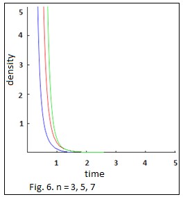
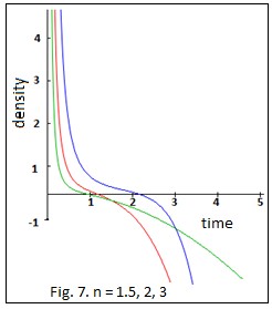
positive for n 3 (Fig.6).
( ) is
We have discussed Bianchi type III cosmological model for two cases (i) Reddy string and (ii) Nambu string. It is found that in both the cases, the model always represent accelerating and decelerating universe under the conditions (33), (34) and (57), (58). It has been shown that in the case of Reddy string and Nambu string, the models are not free from singularities. It is reasonable to say that cosmological model is required to explain acceleration in present universe. Therefore, our theo- retical models are in agreement with recent observations (Perlmutter et al.1999; Garnavich et al.1998; Riesset al.1998; Schmidt et al.1998). Further under the constraint
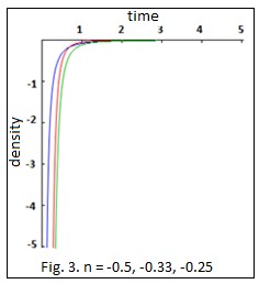
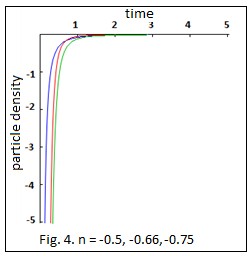
1, K 1, M 1 for Reddy string, in the presence of
magnet, the particle density is negative in 1 n 0
and in
IJSER © 2012
International Journal of Scientific & Engineering Research, Volume 3, Issue 11, November-2012 7
ISSN 2229-5518
![]()
the absence of magnet in 1 n 1
2
(Fig. 3 and Fig. 4). For
[22] Wang, X.X.:Chin. Phys. Lett.23, 1702 (2006).
[23] Zel’dovich, Ya.B. Mon Not. R.Astron. Soc.192, 663 (1990).
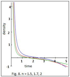
Nambu string under the constraint 1, K 1, in the pres-
ence of magnet, the energy density is negative in n 3 and in the absence of magnet in n 2 (Fig. 7 and Fig. 8).
[1] Bali, R., Upadhaya, R.D.: Astrophysics and Space-Science
[2] Banerjee, A., Sanyual, A.K., Chakraborty, S.: Pramana –
J.Phys. 34, 1 (1990)
[3] Chakraborty, S.: Ind. J. Pure andAppl.Phys.29, 31 (1991)
[4] Garnavich, P.M.: Astrophys. J. 493, L53 (1998).
[5] Kibble, T.W.B., J.Phys.A: Math.Gen.9, 1387 (1976).
[6] Krori, K.D., Chaudhary, T., Mahanta, C.R., Mazumdar, A.: Gen. Relativity and Grav. 22, 123 (1990)
[7] Letelier, P.S.: Phys. Rev.D 20, 1294 (1979) [8] Letelier, P.S.: Phys Rev.D 28, 2414 (1983)
[9] Melvin, M.A.: Ann.New York Acad.Sci.262,253 (1975) [10] Perlmutter, S.: Astrophys. J. 517, 565 (1999)
[11] Riess, A.G.: Astron. J. 116, 1009 (1998)
[12] Roy, S.R., Banerjee, S.K.: Class Quantum Grav.11, 1943 (1995)
[13] Schmidt, B.P.: Astrophys. J. 507, 46 (1998)
[14] Shri Ram, Singh, T.K.: Gen. Relat. Gravit. 27 (11), 1207 (1995)
[15] Singh, G.P., Singh, T.K.: Gen. Relat. Gravit. 31 (3), 371
(1999)
[16] Stachel, J.: Phys. Rev.D21, 217 (1980).
[17]Tikekar, R., Patel, L.K.: Gen. Relativity & Grav.24, 397 (1992).
[18] Upadhaya, R.D., Dave, S.: Brazilian Journal of Physics, 38,
4 (2003)
[19] Wang, X.X.: Astrophysics and Space-Science 293, 933 (2000).
[20] Wang, X.X.: Chin. Phys. Lett.21, 1205 (2004).
[21] Wang, X.X.: Chin. Phys. Lett.22, 29 (2005).
IJSER © 2012