International Journal of Scientific & Engineering Research, Volume 2, Issue 10, October-2011 1
ISSN 2229-5518
Availability Analysis of a System Having Two Units in Series Configuration with Controller and Human Failure under Different Repair Policies
V.V.Singh, Dilip Kumar Rawal
Abstract - This paper deals with the availability analysis of a complex system that consists of two subsystems namely subsystem 1 and subsystem
2.Subsystem 1 is working under k-out of –n good policy and subsystem 2 has two identical units in parallel configuration. Controller for proper functioning controls the subsystems 1. All failure rates are constant and follow exponential distribution but repairs follow general and Gumbel-Houggard family copula distribution. The system is analyze by supplementary technique by evaluating varies measures of reliability such as state transition probability, MTTF, etc. Some computations are taken as special cases by evaluating availability of system and profit analysis
Keywords:Controller, Gumbel-Hogaard family copula, human failure, MTTF, k-out of n policy, supplementary variable, profit function
———————————————————
Many author including [1,6,8] has discuss reliability of complex systems by taking varies failure and one repair policy. By thinking about present scenario and complexity of advance technology and modern demand of electronic equipments one need to study of a controller, which is used in, varies electronic devices and systems.
In this paper author has considered a complex system, which consists of two subsystems 1 and subsystem 2. The subsystem
1 follows (k- out of -n good) policy, the subsystem 2 has two identical units in parallel configuration. Both subsystems are connected in series. The subsystem1 controlled by a controller. The system can fail in following situations: (1) more than k units of subsystem 1 has failed but both units of subsystem 2 are in good working condition, (2) Human failure occur in system, (3) Controller of subsystem 1 fails, (4) Both units of subsystem 2 fail. The system will be in minor partial failure in following situations: (1) All units of subsystem 1 are good and one unit of subsystem 2 has failed, (2) At least k units of subsystem 1 are good and one unit of subsystem 2 has failed.
Many authors have considered reliability and MTTF of a complex system, with different types of failures and one type of repair. However, they did not consider one of the important
aspects of repair between two transitions states i.e. how system will be behaving when there are two different types of repair possible between two adjacent states, which seems to be possible in many engineering systems. When this possibility exists, reliability of the system can be analyzed with the help of copula [7]. The authors [10] have discussed the availability of a system having three units under preemptive resume repair policy using copula in deliberately failure state. Therefore, in contrast to the earlier models, here author has considered a model in which he tried to address the problem where two different repair facilities are available between adjacent states i.e. the initial state and complete failed states. All failure rates are assumed to follow negative exponential distribution. The repairs follow general and Gumbel-Hougaard family copula distributions. In present paper, S0 is state where the system is in good working condition. S1,S3,S4 are state where the system is in partial or degraded mode and states S2, S5, S6, S7,and S8 are states where the system is in completely failure mode. When the system is in degraded mode, the general repaired is employed but whenever the system is in completely failure mode, the system is repaired by Gumbel- Haugaard family copula [7]. The system is analyzed by supplementary variable technique and varies measures of reliability has been discussed and some particular cashes are also taken to highlight the result. The results are demonstrated by graphs and conclusions are drown by graphs.
Author Dr.V.V.Singh is a professor in department of mathematics at DIT School of engineering Greater Noida
(Gautam Budha Nagar)mtu (India) Email:singh_vijayvir@yahoo.com ,Ph.01202390983
IJSER © 2011
International Journal of Scientific & Engineering Research, Volume 2, Issue 10, October-2011 2
ISSN 2229-5518
Coauthor Dilip Kumar Rawal is a research in mathematics department at Mewar university Chittorgarh Raj.
(India)Email:diliprawa05@gmail.com
ASSUMPTION
The following assumptions are taken throughout the discussion of model.
(1) Initially the system is in S0 state and all units of subsystem
1 and 2 are in good working condition.
(2) The sub system 1 works successfully till at least k- units of it is in good working condition.
(3) Subsystem 1 fails if more than k units fail.
(4) Sub system 2 work successfully if at least one unit is good. (5) Subsystem 2 may repair when one unit fails or both unit
fail or controller fails.
(6) All failure rates are constant and follow exponential distribution.
(7) Minor partial failure is repaired by general time distribution. (8) Human failure /complete failure system need fast
repairing (Gumbel-Hougaard) family copula.
(9) Repaired system works like a new and repair did not damage anything.
(10) Only one change is allowed at a time in the transitio
i | Failure rate of 1 unit in sub system 1. |
1 / 2 | Failure rates of subsystem 1 such that at most k unit /more than k units failed during operational mode . |
h / c | Failure rates due to human failure/controller of subsystem. |
| Failure rates of sub system 2. |
(x) | Minor repair rates for state S1, S3 and S4. |
![]()
IJSER © 2011
International Journal of Scientific & Engineering Research, Volume 2, Issue 10, October-2011 3
![]()
ISSN 2229-5518
C (u1, u 2 ( x)) 0 ( x) exp[ x
{lo
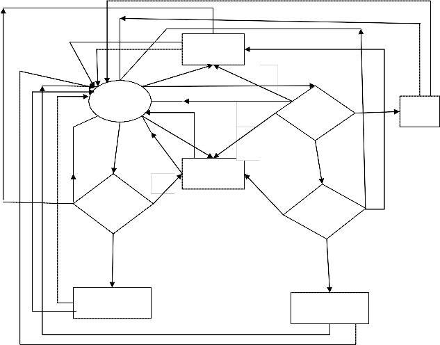
State transition of model
ex
ex
h
P0(t)
(x)
h
P8(x,t)
h
1
( x) 1
(x)
2
P4(x,t)
ex
(x)
P7(x,t)
( x)
c
c
P1(x,t) P2(x,t)
2
(x)
P3(x,t)
(x)
ex S
P6(x,t)
(
ex
![]()
(x)
P5(x,t)
![]()
![]()
Good Degraded Completely failed
IJSER © 2011
International Journal of Scientific & Engineering Research, Volume 2, Issue 10, October-2011 4
ISSN 2229-5518
FORMULATION OF MATHEMATICAL MODEL
By probability of considerations and continuity arguments, we can obtain the
following set of difference differential equations governing the present
mathematical model.
![]()
t 1 C h 2 P0 (t) (x)P1 (x,t)dx (x)P4 (x,t)dx
![]()
![]()
t x C h
( x) P3 ( x, t) 0...(4)
0 0
![]()
![]()
t x C h ( x) P4 ( x, t) 0...(5)
1 /
( x)P3 ( x, t)dx exp[ x
{log ( x)} ]
P7 ( x, t )dx
![]()
![]()
0 0
exp [ x {log (x)} ]1 / P (x,t) 0...(6)
exp[ x
{log ( x)}
]1 /
P6 ( x, t)dx
t x
1 /
![]()
![]()
0 t x exp [ x
{log ( x)} ]
P6 ( x, t) 0...(7)
1/
![]()
![]()
exp [ x
{log ( x)} ]1 / P ( x, t) 0...(8)
exp [ x
0
{log ( x)} ]
P8 ( x, t )dx
t x 7
1 /
exp [ x
{log ( x)} ]1 / P ( x, t) 0...(9)
exp[ x
0
{log ( x)} ]
P5 ( x, t)dx
![]()
![]()
t x 8
exp [ x
0
{log ( x)}
]1 /
P2 ( x, t )dx...(1)
BOUNDARY CONDITIONS
P1 (0, t) 1 P0 (t)...(10)
![]()
![]()
t x 2 C h 2 (x) P1 (x, t) 0....(2)
P (0, t)
P (t)...(11)
2
1 2 0
1 /
P3 (0, t) 21P0 (t)...(12)
![]()
![]()
t x exp[ x
{log (x)} ]
P2 (x, t) 0...(3)
IJSER © 2011
International Journal of Scientific & Engineering Research, Volume 2, Issue 10, October-2011 5
ISSN 2229-5518
P4 (0, t) 2P0 (t)...(13)
P9 (0, t) h (1 1 )(1 2)P0 (t)...(17)
P (0, t) 22 P (t)...(14)
INITIALS CONDITIONS
P6 (0, t) 2
P0 (t)...(15)
P0 (0) 1and other state probabilities are zero at t
P7 (0, t) C (1 1 )(1 2)P0 (t)...(16)
= 0 ...(18)
SOLUTION OF THE MODEL
![]()
![]()
1 /
P5 (x, s) exp [ x
{log (x)} ]
dx P3 (x, s) (x)dx..(19)
0 0
Taking Laplace transformation of equations (1)-(17) and using![]()
equation (18), we obtain ![]()
s x 2 2 C h ( x) P1 ( x, s) 0...(20)
![]()
![]()
s 1 C 2 h P0 (s) 1 P1 (x, s)(x)dx
![]()
![]()
0 s
exp [ x
{log ( x)} ]1 / P ( x, s) 0...(21)
![]()
P ( x, s) exp [ x
0
{log ( x)} ]1 / dx
x
![]()
![]()
s x C h ( x) P3 ( x, s) 0...(22)
![]()
P4 (x, s) (x)dx
0
![]()
P (x, s) exp [ x {log (x)} ]1 / dx
![]()
0
![]()
s x C h ( x) P4 ( x, s) 0...(23)
![]()
P (x, s) exp[ x {log (x)} ]1 / dx
0 0
![]()
P (x, s) exp[ x {log (x)} ]1 / dx
![]()
1 /
![]()
s x exp [ x
{log ( x)} ]
P5 ( x, s) 0...(24)
![]()
1 /
![]()
![]()
P3 (0, s) 21 P0 (s)...(30)
![]()
s x exp [ x
{log ( x)} ]
P6 ( x, s) 0...(25)
1 /
![]()
s x exp [ x
![]()
{log (x)} ]
P7 ( x, s) 0...(26)
![]()
P4 (0, s) 2P0 (s)...(31)
![]()
1 /
![]()
![]()
P (0, s) 22 P (s)...(32)
![]()
s x exp [ x
{log ( x)} ]
P8 ( x, s) 0...(27)
![]()
![]()
P (0, s) 22 P (s)...(33)
6 0
![]()
![]()
P1 (0, s) 1 P0 (s)...(28)
![]()
![]()
P2 (0, s) 12 P0 (s)...(29)
IJSER © 2011
![]()
![]()
P7 (0, s) C (1 1 )(1 2)P0 (s)...(34)
![]()
![]()
P8 (0, s) h (1 1 )(1 2)P0 (s)...(35)
International Journal of Scientific & Engineering Research, Volume 2, Issue 10, October-2011 6
ISSN 2229-5518
Solving (19) -(27) with the help of (27) -(35), one may get![]()
P0 (s)
1
![]()
D(s)
...(36)
![]()
P1 (s)
![]()
1
D(s)
(1 S (s 2 2 C h ))
(s 2 2 C h )
...(37)
(1 S
![]()
1/ (s))
![]()
P2 (s)
![]()
12
D(s)
exp[x {log ( x )} ]
s
...(38)
D(s) s 1 C h 2 {1S (s 1 C h 2) (C (1
![]()
2
(1 S (s C h ))
(1 2))S 1 / (s)
exp[x {log ( x)} ]
P3 (s)
![]()
![]()
1
D(s)
(s C
h )
...(39)
(C
(1 1
)(1
2))S
exp[x
{log ( x)}
1 / (s)
]
![]()
2 (1 S (s C h )
P4 (s)
![]()
![]()
D(s)
(s C h )
...(40)
h (1
1 )(1 2
)S
exp[x
{log ( x )}
1 / (
]
s)
![]()
P5 (s)
2 2
![]()
D(s)
(1 S 1/ (s))
exp[x {log ( x )} ]
s
...(41)
2S
(s C
h
) 2
1 S
(s C
h )
![]()
P6 (s)
22
D(s)
(1 S 1/ (s))
![]()
exp[x {log ( x )} ]
s
...(42)
12 Sexp[x {log ( x)} ]1 / (s)
![]()
P7 (s)
![]()
C (1 1 )(1 2) (1 Sexp[x {log ( x)} ]1/ (s))
...(43)
22 S
exp[x {log ( x)}
1 / (s)}...(45)
]
D(s) s
![]()
P8 (s)
![]()
h (1 1 )(1 2) (1 Sexp[x {log ( x)} ]1/ (s))
..(44)
D(s) s
The Laplace transformations of the probabilities that the system is in up (i.e. either good or degraded state) and
failed state at any time
are as follows:![]()
![]()
![]()
![]()
![]()
Pup (s) P0 (s) P1 (s) P4 (s) P3 (s)
(1 S (s C h )
(1 S (s C h ))
1 1 (1 S (s 2 2 C h ))
![]()
(s C h )
![]()
(s C h )
![]()
![]()
D(s) 1
(s 2 2 C h )
..........(46)
![]()
![]()
![]()
![]()
![]()
![]()
Pfailed (s) P2 (s) P5 (s) P6 (s) P7 (s) P8 (s)
IJSER © 2011
International Journal of Scientific & Engineering Research, Volume 2, Issue 10, October-2011 7
ISSN 2229-5518
(1 S
1/ (s)) 2
2 (1 S
1/ (s))
2 (1 S
1/ (s))
![]()
12
D(s)
exp[x {log ( x)} ]
s
![]()
1
D(s)
exp[x {log ( x)} ]
s
![]()
D(s)
ex p [x {lo g ( x )} ]
s
![]()
h (1 1 )(1 2 ) (1 S ex p [x {lo g ( x )} ]1/ (s))
...(47)
D(s) s
PARTICULAR CASES
When repair follows exponential distribution. Setting
For, t= 0, 10, 20, 30, 40, 50, 60, 70, 80, 90.... One may get different values of Pup(t) as shown in Table
1.If there are n identical units in subsystem in
parallel configuration and
![]()
S 1 / (s)
![]()
exp[x
{log (x)} ]1 /
1 ki 2
(k i)i
exp[ x {log ( x )} ]
s exp[x
{log (x)} ]1 /
![]()
, S
(s)
![]()
s
, in equation (47) and
2 2 2 2 2
(1) Setting the values of different parameters
as λ1=0.05, λ2=0.06, λC= 0.01, λh= 0.01, λ
= 0.005, = 1, θ = 1and x = 1 then taking
inverse Laplace transform, one can obtain,
![]()
Pup
(t) 0.012358e(2.1524t ) 0.0051717e(1.1505t )
0.000414e( 1.0559t ) 0.99285e( 0.0024957t ) ..(48)
(II) Setting the values of different parameters
as λ1 = 0.06, λ2 = 0.07, λC= 0.01,
![]()
Pup (t)
0.01296e
( 2.7541t )
0.0064844e
( 1.1688t )
0.000025851e( 1.0560t ) 0.99355e( 0.002325t ) ...(49)
IJSER © 2011
International Journal of Scientific & Engineering Research, Volume 2, Issue 10, October-2011 8
ISSN 2229-5518
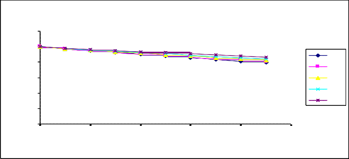
1.2
1
0.8
0.6
0.4
0.2
Pup PuP Pup Pup Pup
0
0 20 40 60 80 100
Setting![]()
exp [ x {log ( x)} ]1 /
![]()
S 1/ (s) ,
one may obtain Table 2 which shows variation of MTTF with respect to λh. Setting 1 0.05, C 0.01, h 0.01and varying λ as 0.01, 0.002, 0.03, 0.04, 0.05, 0.06, 0.07, 0.08, 0.09 in (50) one may obtain Table 2, which reveals variation of MTTF
with respect to λ.
exp[x {log ( x )} ]
![]()
![]()
S (s)
s
s exp [ x {log ( x)} ]1 /
C 1
and taking all repairs to zero in equation
(51a). Taking limit as s tends to zero one can obtain the MTTF
as:![]()
M .T .T .F. lim P
![]()
(s) 1
… (50)
s0 up
(1 C h 2)
Setting C
0.01, CB 0.02, h 0.01, 0.005
and
varying λ1 as 0.01, 0.02, 0.03, 0.04, 0.05, 0.06, 0.07, 0.08, 0.09 in (50) one may obtain Table 2 which demonstrates variation of
MTTF with respect toSetting
1 0.05, h 0.01, 0.005
and varying λc as 0.01,
0.02, 0.03, 0.04, 0.05, 0.06, 0.07, 0.08, 0.09 in (50) one may obtain Table 2 which demonstrates variation of MTTF with respect to λc.
Setting 1 0.05, C 0.01, 0.005 and varying λh
as 0.01, 0.02, 0.03, 0.04, 0.005, 0.06, 0.07, 0. 08, 0.09 in (50)
IJSER © 2011
International Journal of Scientific & Engineering Research, Volume 2, Issue 10, October-2011 9
ISSN 2229-5518
(a) Let the failure rates of system be λ1 = 0.05, λh= 0.001,
30 λ2 = 0.06, λC= 0.01,
20 λ = 0.005, mean time to repair of be
x 1, 1,(x) 1 . Setting
10
(x) 1, and
![]()
exp [ x {log
( x)} ]1 /
A
MTTF λC MTTF λ
S (s)
1 / s exp [ x {log
( x)} ]1 /
0
0 0.02
MTTF0.04Λh
0M.06TTF Λ10.08 0.1
ex p [x {lo g ( x )} ]
A
![]()
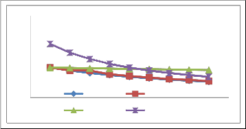
Table and Failure 2 for failure rate v/s MTTF
, S
(s)
s
![]()
in equation (46) and taking inverse
Laplace transform, one can obtain (51).
Let the service facility be always available, then expected profit during the interval [0, t] is
t
E p (t ) K1 Pup (t )dt K 2 t
0
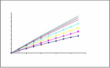
where K1 and K2 are revenue service cost per unit time . Hence
E p (t ) K1
(0.005516e( 2.760 7t )
0.00090376e( 1.222 7t ) 0.000021733e( 1.056 3t ) () 0.001557 9t
639.21e
639.21) K 2t....(51)
Setting K 1 = 1and K 2 = 0.5, 0.4, 0.3, 0.2, 0.1, 0.05, 0.01 respectively and varying t =0, 10, 20, 30, 40, 50, 60, 70, 80,
90,......one get Table .
Tables 1 and Fig. 1 provide information how availability of the complex repairable system changes with respect to time when failure rates are fixed at different values. When failure rates are fixed at lower values λ1= 0.05, λ2 = 0.06, λC= 0.01, λ = 0.005, λh= 0.001, availability of the system decreases and probability of failure increase, with passage of time and ultimately becomes steady to the value zero after a sufficient long interval of time. Hence one can safely predicts the future behavior of
complex system at any time for any given set of parametric
IJSER © 2011
International Journal of Scientific & Engineering Research, Volume 2, Issue 10, October-2011 10
ISSN 2229-5518
values, as is evident by the graphical consideration of the model.
Tables 2, and yield the mean-time-to-failure (MTTF) of the system with respect to variation in λ1, λC,,λh and λ respectively when other parameters have been taken as constant.
When revenue cost per unit time K1 fixed at 1, service cost K2
= 0.5, 0.4, 0.3, 0.2, 0.1, 0.05, 0.01, profit has been calculated and results are demonstrated by graphs. One can observed that as service cost decreases profit increases.
The study shows that incorporation of copula improves the reliability of the system significantly.
The authors wish to thank Dr.S.B .Singh, Dr. Mangeyram and Professor C.K.Goel for insists us to continuing associate with research work and helping at varies stages. Dr.Singh have published number of papers in varies repute international journals.
(1).A.K. Govil, Operational behaviour of a complex system having shelf-life of the components under preemptive-resume repair discipline, Microelectronics &Reliab.,(1974), 13, 97-101.
(2).F. Lindskog, Modelling dependence with copulas, Risklab report, ETH, Zurich (2000).
(3).Heinrich Gennheimer, Model Risk in Copula Based Default Pricing Models, Working Paper Series, Working Paper No. 19, Swiss Banking Institute, University of Zurich and NCCR FINRISK (2002).
(4).Lirong Cui and Haijun Li., Analytical method for reliability and MTTF assessment of coherent systems with dependent components, Reliability Engineering & System Safety (2007), 300-
307.
(5).M. R. Melchiori, Which Archimedean copula is right one?,
(6).P.P. Gupta and M.K. Sharma, Reliability and M.T.T.F evaluation of a two duplex-unit standby system with two types of repair, MicroelectronReliab. (1993), 33(3): 291-295.
(7).R.B. Nelsen, An Introduction to Copulas (2ndedn.) (New York, Springer, 2006).
(8).Singh, S.B.,Gupta. P.P and Goel.C.K : ‘Analytical study of acomplex stands by redundant systems involving the concept of multifailure-human failure under head-of-line repair policy. Bulletin of pure and applied sciences Vol. of 20 E(No.2) 2001; pp 345-351.
(9).Singh, S.K.; Singh, R.P.; Singh, R.B.: ‘Profit evaluation in two unit cold standby system having two type of independent repair facilities’, IJOMAS Vol. 8, 277-288 (1992).
(10).Singh,V.V,SinghS.B,Mangeyram,Goel C.K ‘Availability analysis odf a system havng three units super priority , priority and ordinary under pree-mptive resume reapir policy’ International journal of reliability and applications Vol 11, No1 ,P P (41-53) (2010).,
IJSER © 2011