International Journal of Scientific & Engineering Research, Volume 4, Issue 4, April-2013 1508

ISSN 2229-5518

Assessing the Validity of Regional Climate

Simulations for Agricultural Impact Assessment: A Case study

C N Tripathi and K K Singh

ABSTRACT

Extensive statistical analyses were performed to test the validity of daily climate simulation by Hadley Center, UK, regional climate model version 2 (HadRM2) for agricultural impact assessment at local level in India. Observed and simulated climatic parameters which are used in crop simulation models for agricultural impact assessment such as daily maximum temperature, minimum temperat ure and rainfall were compared in terms of average and standard deviation, maximum and minimum values. Correlation between observed and simulated data were also computed in addition to annual variations in maximum temperature and minimum temperature in observed and simulated climate. Results indicate considerable deviations in the statistical properties of the simulated climate as compared to that of observed climate. Observed daily and annual variability in these climatic parameters is also not adequately replicated in simulated climate. Therefore these simulations can not be used directly into crop simulation models to be acceptable for realistic agricultural impact assessment. However some approaches may be developed where in these simulated climatic information can be applied for agricultural impact assessment. First approaches may be to use observed climate information int o impact assessment models as baseline climate and creating the required future climate information by enforcing the baseline observed climate by changes derived from the model simulations of the pr esent and future climate. The second approach may be to us e climate model simulated data for both periods (present and future) into impact assessment models then the difference between two responses will represent the impact of climate change in that sector. Third approach can be to use the long term monthly mean of simulated climatic parameters into properly calibrated weather generator to generate the realistic daily weather data to be used in imp act assessment models.

Key words: Climate, Models, Regional, Simulation, Variability

1. Introduction

Anthropogenic CO2 emissions due to human activities are virtually certain to be the dominant factor causing the observed global warming and climatic changes due to increased radiative forcing. The complex interactions of the different components of the climate system (atmosphere, hydrosphere, cryosphere, biosphere, etc.) are most comprehensively modeled using coupled atmosphere- ocean General Circulation Models (GCMs). These interactions are expressed in terms of a set of dynamic equations for the atmosphere, oceans and ice along with appropriate equations for the laws of conservation and state, for selected constituents (such as water substance, CO2 and the ozone in the air and salt and trace substances in the ocean. Today, many climate research institutions all over the world are pursuing research programs and
-------------------------------------------------------------------

C N Tripathi is Associate Professor at1 Department of Environmental Engineering, Hindustan College of Science and Technology, Farah Mathura, India,

E mail: cntripathi01@gmail.com

K K Singh is Sciebtist E at Agromet Servic es, Mausam Bhawan, Lodi

Road, New Delhi-110003

Email: Kksingh2022@gmail.com

projects for better understanding of the present day climate and the future climate change through modeling and other approaches. As a result many Global and regional climate models are now available and are being improved further - in their resolution as well as in their parameterization scheme. Now the improved understanding of the effect of the aerosols in addition to the greenhouse gases on the climate are also being taken into account. To project the future trajectory of greenhouse gases different emission scenarioe have been developed such as SRES ‘Marker’ emission scenarios namely A1, A2, B1, B2 (IPCC 2001) and
IS92 (IPCC 1994). Each scenario describes different world

IJSER © 2013

http://www.ijser.org

International Journal of Scientific & Engineering Research, Volume 4, Issue 4, April-2013 1509

ISSN 2229-5518

evolving through the 21st century and leads to different
greenhouse gas emission trajectories.
On a global scale, a number of climate models (developed by different scientific groups in the world) have shown Model may perform poorly in model validation on regional scale. In order to overcome these limitations high- resolution Regional Climate Models (RCMs) are now being developed which are driven at its boundaries by the output derived from a GCM. RCM is a limited area high-resolution climate model that is embedded in a coarse resolution GCM over the area of interest. At the lateral boundaries, either two-way or one-way interacting nesting can be employed. The two-way nesting technique allows the interaction of the regional and global climate models iteratively and therefore requires simultaneous integration of the two models. In the one way nesting techniques the initial and lateral boundary conditions needed to run the regional model are provided by the output of the GCM simulation. Regional climate models attempt to capture regional details in surface climatic characteristics as forced by regional details such as topography, lakes, coastline and land use distribution Leung et al 2003, 2005). Giorgi et al., (2001) has proposed more systematic and wider applications of RCMs to adequately assess their performances and uncertainties in producing the regional climate information.
Climate change will affect all economic sectors to some degree, but the agricultural sector is perhaps the most sensitive and vulnerable. Agriculture is affected by variations in climatic factors such as CO2 concentration, temperature, precipitation, radiation, humidity, wind speed and frequency and severity of extreme events like droughts, floods, hurricanes, windstorms, and hail. Most crop simulation models which are used to simulate the impact of climate change and variability require weather data at a higher spatial resolution of the order of 50KM by
50 KM or even more and at daily temporal resolution.
Given the potential importance of regional climate changes for the development of national policies, and the impacts of extreme weather events such as droughts, floods, and hurricanes on agriculture, it is necessary to evaluate the climate Simulation by Regional Climate Models at daily and sub daily temporal resolution and at local level. A number of attempts have been made in the past to demonstrate the capability of regional climate models embedded in General Circulation model in simulation the
considerable improvements in simulating the present day
climate. However, the regional climates by these global models lack the finer scale details and therefore these
Indian Climatology (Jones et al., 1995; Bhaskaran et al.,
1996; Vernakar et al., 1999; Lal ,M 2000;sh et al., 2006; Mukhopadhyay et al., 2010, Bhate et al., 2012). However non of these attempts were applied to test the daily simulation of climate at a very high resolution of 50 KM by
50 KM spatial resolution which is very important in view of
many agricultural and hydrological impact models use weather data at such higher resolution only. Keeping this in mind a study is presented here to test the ability of daily climate simulation by Hadley Center, UK, regional climate model version 2 (HadRM2) at 50 KM by 50 KM resolution to find its applicability in crop simulation models for agricultural implications over Indian subcontinent. Details methodology and data used are discussed in the following section.

2. Materials and Methods

2.1. Hadley Center Regional Climate Model Version 2 (HadRM2)

The RCM (HadRM2) is a high-resolution limited area atmospheric model driven at its lateral and sea surface boundaries by output obtained from HadCM2 integration. The formulation of HadRM2 is identical to the atmospheric component of HadCM2(Jones et al., 1995; Bhaskaran et al.,
1996). Apart from details concerning diffusion and filtering,
both models use 19 hybrid coordinate vertical levels and
regular latitude-longitude horizontal grids. The grid spacing in HadCM2 is 2.5° X 3.75° and 0.44° X 0.44° in HadRM2 which is kept quasi-regular over the region of interest by shifting the coordinate pole. The time steps are 30 and 5 minutes respectively. General details of the RCM formulation and the one-way nesting technique may be found in Jones et al., 1995, whilst Bhaskaran et al., 1996 provide specific information on the RCM set up for the Indian monsoon region. Though higher resolution regional climate models are now available now, but the availability of simulated climate data for all the region of India is limited by cumbersome exercise and computer power required. Therefore at first stage of we have used the climate data as simulated by Hadley Center Regional Climate Model Version 2 (HadRM2)

IJSER © 2013

http://www.ijser.org

International Journal of Scientific & Engineering Research, Volume 4, Issue 4, April-2013 1510

ISSN 2229-5518

2.2. General Climatic Features over Indian

Subcontinent

In India, the two monsoon seasons (the southwest monsoon from June to September and the northeast monsoon from November to December bring rains many a times in intensities and amounts sufficient to cause serious floods creating hazardous (and often disastrous) situations. Moreover, India also experiences cyclonic storms in the pre- monsoon months (April-May) and post-monsoon months
(October-November) which also cause large-scale inundation and destruction.
The long-term average annual rainfall for the country as a whole is 116 cm, the highest for a land of comparable size in the world. But this rainfall is highly variable in both time and space. The maximum rainfall occurs in July and August, during the four-months (June to September) of the southwest monsoon season. There are considerable intra-
seasonal and inter-seasonal variations as well. The summer monsoon rainfall oscillates between active spells with good

monsoon (above normal) on all India basis and weak spells

normal) rain occur on all India basis for a few days at a stretch. The average seasonal summer monsoon rainfall in India is about 85 cm with a standard deviation of about
northeastern States, the Western coast and the Ghats receive more than 100 cm of rainfall. The heavy rainfall in the northeastern States, West coast and the Ghats and the sub-mountainous regions are influenced by the orography. The peninsular India south of 15°N gets less than 50cm of rainfall and extreme southeast peninsula gets the lowest rainfall. The west and the northwest regions of the country receive about 50 cm of rain in the monsoon season. The rainfall decreases rapidly to less than 10 cm in the western Rajasthan. Regions above 50 cm of rainfall in the monsoon season are classified as wet and that less than 50 cm as dry parts of the country.

2.3. Validating the Simulated Climate

Simulated climate variables relevant to agricultural implications were evaluated against observations at six locations situated in six different geographic regions in India namely Ludhiana (North India), Coimbatore (South India), Anand (West India), (Power Kheda (Central India), Pusa (East India) and Jorhat (North-East India) in India. Coordinate of these locations are shown in Fig. 1.

2.3.1. Simulated Base line and Future Climate Data Control and anomaly GCM climate simulation had each been carried out for 21 years by Hadley Center of climate research UK. CO2 is held constant in the control simulation at present day values. The anomaly integration (GHG) has CO2 increasing by 1% per year (compound) and is initialized after 50 years of increasing CO2 concentrations, in the year 2040. The nested RCM simulations were integrated over the same periods with the first year disregarded. The data generated in these transient experiments were obtained from “Hadley Center for Climate Prediction” U.K. at a resolution of 0.44° X 0.44°

latitude by longitude grid points for whole India. The daily weather data on maximum and minimum temperature and
rainfall for six selected locations in India were obtained by taking weighted mean of values of respective weather parameter at four nearest grid points surrounding these locations. These data for present/control (1990s) and future/anomaly (2050’s) climate also indicate the nature of change in climate variability in addition to change in climatic mean.

2.3.2. Observed Weather Data

For comparing the statistical properties of the simulated climatic data with the corresponding observed data the daily observed weather data on maximum and minimum temperature and rainfall for 19 years (15 years for some of the locations) for the period 1980-1999 (1985-1999 for some of the locations) have also been collected from India Meteorological Department Pune, for six selected locations as shown in Table 1.

Table 1

Co-ordinates and Weather Data Period for

Selected Locations in India

IJSER © 2013

http://www.ijser.org

International Journal of Scientific & Engineering Research, Volume 4, Issue 4, April-2013 1511

ISSN 2229-5518

2.3.4. Comparison of Statistical Properties of observed and Simulated Climate

Extensive statistical analyses were performed to test the ability of the HadRM2 in simulating the features (mean and variability) observed in maximum temperature, Minimum temperature and rainfall in observed climatology for all the six locations for which the daily observed and simulated data were available. The statistical properties of these
parameters such as average and standard deviation, maximum and minimum values in both observed and
simulated data for whole simulation duration were compared. scattered chart were also plotted to find the correlation coefficient between the simulated and observed daily data. Annual variation in maximum temperature and minimum temperature of observed and simulated values were also compared. Our findings on these analysis’s is discussed in the next section.

3. Results and Discussion

3.1. Observed and Simulated Maximum Temperature

Scattered diagram plotted between daily observed and daily simulated maximum temperature for six selected locations of India are shown in Fig. 1. Annual variation in observed and simulated maximum temperature is shown in Fig. 2. Detail interpretation of Fig. 1 and Fig. 2 is summarized in Table 2 where statistical properties of observed and simulated data are shown. Table 2 shows that the simulated maximum temperature is not a good representation of observed maximum temperature for most of the locations in India, except for some degrees in North India . Average values of observed an simulated max
temperature in Table 2 show that the observed annual maximum temperature is overestimated at most of the locations in North, North East and East India where as it is underestimated at most of the locations in South, West and Central India. Variability of daily maximum temperature (as indicated by the values of standard deviations in Table
2) was in general higher in simulated climate than that in
observed climate. Maximum daily value of maximum temperature occurred during simulated period was more in simulated temperature than in observed temperature for most of the locations except for the locations in South India. However minimum values of the maximum temperature occurred during the simulation period was lower in simulated climate than that in observed climate.

Table 2: Comparison of Observed and Simulated Maximum Temperature

Station Equation of Best fit line

Cor.Co eff

Average. St. dev Max value Min value

Obs Sim Obs Sim Obs Sim Obs Sim

Ludhiana (North

India)

y=1.007x+2.75 0.80 29.6 32.6 7.3 9.1 46.6 52.1 9.2 2.9

Coimbatore

(South India)

y=0.4498x+18.35 0.39 32.0 32.7 2.7 3.1 39.5 40.2 22.2 21.8

Anand (W est

India)

y=0.920x+1.38 0.65 33.5 32.2 4.24 6.03 44.7 48.0 15.3 12.9

Powerkheda

(Central India)

y=0.699x+9.45 0.67 31.0 31.0 5.6 5.9 49.0 47.4 14 12.6

Pusa (East India) y=7.741x+9.91 0.60 31.0 33.1 5.0 6.2 44.0 50.8 12.8 10.0

Jorhat (North-East

India)

y=0.55x+13.46 0.46 28.3 29.0 4.1 4.9 37.6 44.0 16.2 10.7

IJSER © 2013

http://www.ijser.org

International Journal of Scientific & Engineering Research, Volume 4, Issue 4, April-2013 1512

ISSN 2229-5518

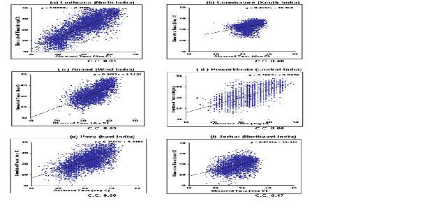
Fig. 1: Comparison of Observed and Simulated Maximum Temperature

IJSER © 2013

http://www.ijser.org

International Journal of Scientific & Engineering Research, Volume 4, Issue 4, April-2013 1513

ISSN 2229-5518

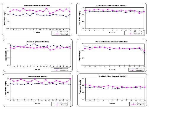
Fig. 2: Observed and Simulated variation in Annual Maximum Temperature

3.2. Observed and Simulated Minimum Temperature Scattered diagram plotted between daily observed and daily simulated maximum temperature for six selected locations of India are shown in Fig. 3. Annual variation in observed and simulated maximum temperature is shown in Fig. 4. Detail interpretation of Fig. 3 and Fig. 4 is summarized in Table 3 where statistical properties of observed and simulated data are shown. Result indicate that model is able to simulate daily minimum temperature in better agreement to observed minimum temperature as compared to that of maximum temperature in different geographic regions (as indicated by correlation coefficient and values of slope and intercept of the best fit line in Fig

3 and Table 3) except for the locations in South India
where comparison is not reasonably good. Fig. 4 and average values of observed an simulated minimum temperature in Table 3 show that the observed annual minimum temperature is under-estimated at most of the locations in North and South India where as it is
overestimated at most of the locations in West India. In
other geographic regions both over and under estimations of observed minimum temperature (depending upon the locations) have occurred in simulated climate. Simulated daily variability of minimum temperature (as indicated by values of standard deviation in Table 3) for the simulated period is in general higher in simulated climate than that in observed climate in the region North, South, East and North East India, where as in general it is lower in simulated climate than that in observed climate in West and Central India. Maximum daily value of minimum temperature occurred in simulated climate for the simulated period were in general more or close to that of observed temperature in North, West and East India where as it were in general lesser or close to that in observed in South, Central and North-East India. However minimum values of the minimum temperature occurred during the simulation period were lower in simulated climate at than that in observed climate in west,

IJSER © 2013

http://www.ijser.org

International Journal of Scientific & Engineering Research, Volume 4, Issue 4, April-2013 1514

ISSN 2229-5518

central and north-east India where as for other region it was more than that in simulated climate.

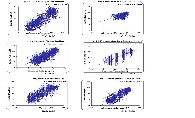
Fig. 3: Comparison of Observed and Simulated Minimum Temperature

IJSER © 2013

http://www.ijser.org

International Journal of Scientific & Engineering Research, Volume 4, Issue 4, April-2013 1515

ISSN 2229-5518

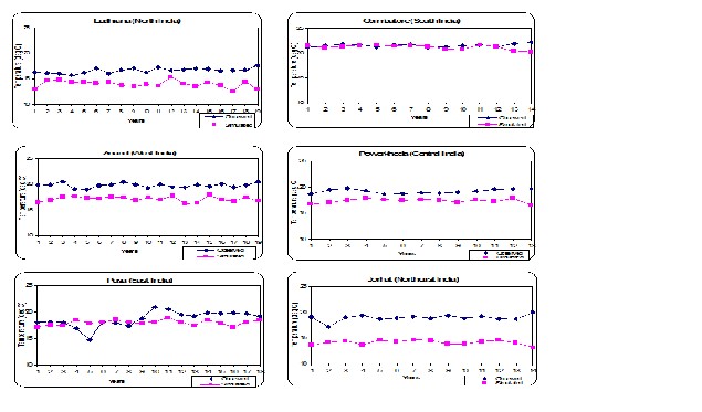
Fig. 4: Observed and Simulated Variation in Annual Mean Minimum Temperature

Table 3 : Comparison of Observed and Simulated Minimum Temperature

Station Equation of best fit line Cor.

Average. St. dev Max value Min value

IJSER © 2013

http://www.ijser.org

International Journal of Scientific & Engineering Research, Volume 4, Issue 4, April-2013 1516

ISSN 2229-5518

3.3. Observed and Simulated Rainfall

Comparison of rainfall in observed and simulated climatic data for six locations situated in six different geographic regions of India are shown in Fig 5. Results of the detail statistical analysis of the observed and simulated data for all the six locations have been summarized in Table 4. Comparisons indicate that the ability of HadRM2 is very- very poor in simulating the observed rainfall in all geographic regions (as indicated by very small values of correlation coefficient and the values of slope and intercept of the best fit line in Fig 5 and Table 4). However average daily rainfall for the simulation period in both simulated and observed climate are very close to each other. Simulated daily variability of rainfall (as indicated by values of standard deviation in Table 4) for the simulated period is in general lower in simulated climate than that in observed climate for all the geographic region of India. Maximum daily value of rainfall occurred in simulated climate for the simulated period were in general less than that in observed rainfall in North, West, Central and East India where as it were in general more or close to that in observed in South, and North-East India. However minimum values of the rainfall occurred during the simulation period were very close to each other in all the geographic regions of India
.Table 4: Comparison of Observed and Simulated Rainfall

IJSER © 2013

http://www.ijser.org

International Journal of Scientific & Engineering Research, Volume 4, Issue 4, April-2013 1517

ISSN 2229-5518

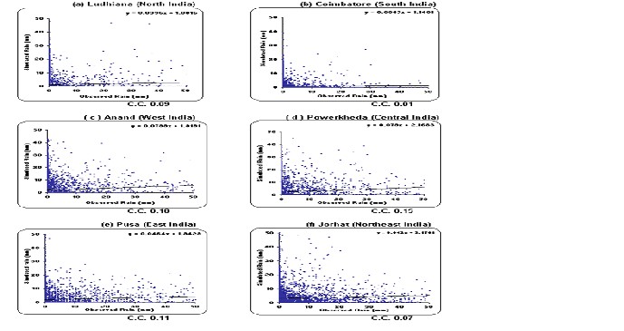
Fig. 5: Comparison of Observed and Simulated Rainfall

These results indicate that in general HadRM2 is not able to
simulate the observed climatology as there is considerable bias in its simulation to be acceptable for realistic agricultural impact assessment. Therefore using these simulation can not be used directly into crop simulation models. However some approaches may be developed where in these simulated climatic information can be applied for agricultural impact assessment of climate change and variability. First approaches may be to use observed climate information into impact
models as baseline climate and creating the required future
climate information by enforcing the baseline observed
climate by changes derived from the model simulations of the present and future climate. Second approach is to use climate model data for both periods (present and future) into impact model then the difference between two responses will represent the impact of climate change in that sector. Third approach can be to use long term monthly mean of simulated climatic parameters into properly calibrated weather generators to generate the realistic daily weather data to be
used in impact assessment models

4. Conclusions

Properly tested daily climate simulations are required to be
used in crop simulation models for realistic agricultural impact assessment of climate change. Though several regional climate models are available which simulate the climate variables at daily and sub daily scales and at very high spatial resolution, but the availability of simulated climate data for all the region of India is limited by cumbersome exercise and computer power required. Therefore as a preliminary exercise an attempt has been made in this study to test the ability of Hadley Center, UK, regional climate model version 2 (HadRM2)
climate simulation at 0.44 X 0.44 latitude by longitude
resolution for agricultural impact assessment at local level in India. These simulated data were easily available from Hadley center UK. Simulated climate variables to be used in crop simulation models for agricultural implications were evaluated against observations at six locations situated in six different geographic regions in India. Extensive statistical analyses have been performed to compare observed simulated daily and annual maximum temperature, minimum temperature and rainfall for these locations. Results indicate

IJSER © 2013

http://www.ijser.org

International Journal of Scientific & Engineering Research, Volume 4, Issue 4, April-2013 1518

ISSN 2229-5518

that in general HadRM2 is not able to replicate the features of observed climatology as there is considerable bias in its
simulation of observed climatology. Therefore these simulation can not be used directly into crop simulation models to be acceptable for realistic agricultural impact assessment. However some approaches may be used where in these simulated climatic information can be applied for agricultural impact assessment of climate change and variability. First approaches may be to use observed climate information into impact assessment models as baseline climate and creating the required future climate information by enforcing the baseline observed climate by changes derived from the model simulations of the present and future climate. The second approach may be to use climate model simulated data for both periods (present and future) into impact assessment models then the difference between two responses will represent the impact of climate change in that sector. Third approach can be to use long term monthly mean of simulated climatic parameters into properly calibrated weather generator to generate the realistic daily weather data to be used in impact assessment models.

Acknowledgments: Authors are highly thankful to India meteorological Department for providing the required observed weather data for the study. Authors are also thankful to the official of Hadley center UK for providing the regional climate simulation over Indian subcontinent.

References

J. Bhate, C.K. Unnikrishnan and M. Rajeevan, “ Regional Climate Simulation of 2009 Indian Summer Monsoon,” Indian Journal of Radio and Space Physics, Vol. 41, pp.
488-500, August 2012 (Journal citation).
B. Bhaskaran, R.G. Jones, J.M. Murphy and M. Noguer, “ Simulations of the Indian summer monsoon using a nested regional climate model: Domain size experiments,” Clim. Dyn., Vol.12, pp. 573�587, 1996 (Journal citation).
J.T. Houghton, J. Bruce, B.A. Callander, E. Haites, N. Harris, H. Lee, K. Maskell, and L.G. Meira Filho (eds.), “Climate Change 1994: Radiative Forcing of Climate Change and an Evaluation of the IPCC IS92 Emissions Scenarios”. Cambridge University Press, Cambridge, United Kingdom and New York, NY, USA, 339 pp, 1994 (Book style with paper title and editor)
Theor Appl Climatol Vol. 86(1-4):161–172, 2006 (Journal citation).
Nakicenovic, N.,J. Alcamo, G. Davis, B. de Vries, J. Fenhann, S. Gaffin, K. Gregory, A. Grübler, T Y Jung, T. Kram, E.L. La Rovere, L. Michaelis, S. Mori, T. Morita, W. Pepper, H. Pitcher, L. Price, K. Raihi, A. Roehrl, H.-H. Rogner, A. Sankovski, M. Schlesinger, P. Shukla, S. Smith, R. Swart, S. van Rooijen, N. V i c t o r, and Z. Dadi (eds.), “ IPCC2000: Emissions Scenarios. A Special Report of Working Group III of the Intergovernmental Panel on Climate Change,” Cambridge University Press, Cambridge, United Kingdom and New York, NY, USA, 599 p, 2000 (Book style with paper title and editor)
M. Lal , and H Harasawa, “ Comparison of the present-day climate simulation over Asia in selected coupled atmosphere-ocean global climate model,” . Journal of the Meteorological Society of Japan, 78(6), 871–879, 2000 (Journal citation).
Leung L. Ruby, Linda O. Mearns, Filippo Giorgi, Robert L. Wilby, “ Regional Climate Research,” Bull. Amer. Meteor. Soc., 84, 89–95, 2003 (Journal citation).
L.R. Leung, Y.H. Kuo, and J. Tribbia, “Research Needs and Directions of Regional climate Modeling Using WRF and CCSM.”Bull. Amer. Meteorol. Soc.,87(12), 1747-1751, 2006 (Journal citation).
P. Mukhopadhyay, S. Taraphdar, , B. N. Goswami, and Krishnakumar, “ Indian Summer Monsoon Precipitation Climatology in a High-Resolution Regional Climate Model: Impacts of Convective Parameterization on Systematic Biases” Wea. Forecasting, 25, 369–387, 2010 (Journal citation).
A D Vernakar and Y Ji, “ Simulation of the onset and intra seasonal variability of two contrasting summer monsoon. Journal Climate (USA), 12, 1707-1725, 1999 (Journal citation).
R.G. Jones, J.M. Murphy, and M. Noguer, 1995: Simulation of climate change over Europe using a nested regional climate model, part I: assessment of control climate, including sensitivity to location of lateral boundaries. Quarterly Journal of Royal Meteorological Society, 121,

1413-1449, 1995 (Journal citation).

SK Dash, MS Shekhar, GP Singh , “ Simulation of Indian summer monsoon circulation and rainfall using RegCM3,”

IJSER © 2013

http://www.ijser.org

International Journal of Scientific & Engineering Research, Volume 4, Issue 4, A pril-2013

ISSN 2229-5518

1519

IJSER 2013

http://www ijser ora