International Journal of Scientific & Engineering Research, Volume 3, Issue 3, March-2012 1
ISSN 2229-5518
Artificial Neural Network Modeling in Hadrons
Collisions
*Moaaz A. Moussa
Buraydah Colleges, Al-Qassim, Buraydah, King Abdulazziz Road, East Qassim University, P.O.Box 31717, KSA.
moaaz2030@Yahoo.com
*Mahmoud Y. El-Bakry
Tabuk University, Faculty of Science, Department of Physics, Tabuk, KSA.
**A. Radi, ***E. El-dahshan
Ain Shams University, Faculty of Science, Department of Physics, Abbassia, Cairo, Egypt.
**The British University in Egypt (BUE).
***Egyptian E-Learning University- 33 El-mesah St., El-Dokki- Giza- Postal code 12611.
M. Tantawy
*Ain Shams University, Faculty of Education, Department of Physics, Roxi, Cairo, Egypt.
Abstract—Evolutions in artificial intelligence (AI) techniques and their applications to physics have made it feasible to develop and implement new modeling techniques for high-energy interactions. In particular, AI techniques of artificial neural networks (ANN) have recently been used to design and implement more effective models. The neural network (NN) model and parton two fireball model (PTFM) have been used to study the charged particles
![]()
multiplicity distributions for antiproton-neutron ( p
n ) and proton-neutron ( p
![]()
n ) collisions at different lab momenta. The neural network model per-
formance was also tested at non-trained space (predicted) and matched them effectively. The trained NN shows a better fitting with experimental data than the PTFM calculations. The NN simulation results prove a strong presence mod eling in hadrons collisions.
Index Terms —. Neural Network Model; Parton Model; Multiparticle Production.
—————————— ——————————
The validity of the mathematical treatment and assump- tions comes from the agreement between the theoretical re- sults and corresponding outcomes from experimental mea- surements. The closest is this agreement the successful is a
4, 5. The results and conclusion of both models are explained in Section 6.![]()
![]()
According to the parton two fireball model [23-25], p n
certain modeling. Models are provided for the hadron struc-
and p
n interaction will be characterized by the impact pa-
ture [1-3]. These include the quark model [4], three fireball model [5], fragmentation model [6,7], and many others. The theories and ideas concerning multiparticle production go back to the late of 1930s with a significant interlude at Fermi's statistical theory of particle production [8]. Multiparticle pro- duction can be also modeled and described efficiently by
rameter and the corresponding overlapping volume. Let us assume that the two interacting hadrons at rest are spheres each of radius (R). Therefore, the two colliding particles can interact strongly when the impact parameter is in the region from 0 → 2R. Therefore, the statistical probability of any im- pact parameter (b) within an interval (db) is given by
studying the multiplicity distribution [9]. Several methods exist which investigate the multiplicity distribution of particles
P(b)db
![]()
bdb
2R2
(1)
at high energy [10-13]. Among these are the multiplicity scal-
ing [10,11], the statistical boot strap model [12], the two
sources model [14], the negative binomial distribution [15],
Let us use a dimensionless impact parameter, X, defined as,![]()
X b
T2hRen, Eq. (1) can be rewritten as,
fireballs [16], strings [17], quark gluon plasma [18,19] and
P(X) dX
![]()
2X dX
(2)
many others.
Where,![]()
![]()
0 X 1
Parallel to the theoretical approach based on different views, development in the artificial intelligence (AI) field has
Now we employ the overlapping volume, V (b) as a clean cut [26] as,
given the neural networks a strong presence in high-energy![]()
![]()
V (b)db (1 3b
3b 2
2
5b3
3
(3)
physics [20-22]. Neural networks are composed of simple in- terconnected computational elements operating in parallel.
In terms of the dimens8iRonle8Rss im32pRact parameter (X), the overlapping volume V ( X ) can be given by,
These artificial neural networks (ANNs) are trained, so that a
particular input leads to a specific target output. The objective
of this paper is to extract the multiplicity distribution of![]()
V(X) = V (1- 0.75X-1.5X2 +1.25X 3).
Then the fraction of partons, interaction may be written as,
(4)
Z ( X ) participating in the
charged particles for p![]()
n collisions at different lab momenta
![]()
Z(X) = V ( X ) = (1 - 0.75X- 1.5X2 + 1.25X 3).
(5)
using PTFM and NNM. Section 2 presents parton two fireball model PTFM at high energies. Section 3 provides the multipar-
According to Eq. (2) aVn0d Eq. (5), the Z -function distribu-
tion can be given by,
ticle production in proton-neutron and antiproton-neutron![]()
P(Z) dz = 2XdX (-2.4375X- 0.75X-1 + 7.125X
0.75X2 - 9.375X3
![]()
4.687X4 )-1.
(6)
collisions using PTFM . The NN model is described in Sections
IJSER © 2012
![]()
![]()
Where, 0 Z 1
http://www.ijser.org
International Journal of Scientific & Engineering Research Volume 3, Issue 3, March-2012 2
ISSN 2229-5518
From Eqs. (2, 5) and using least square fitting technique
Where, N is the number of pairs of created particles from
(LSFT), Z -function distribution can be written in the follow-
one fireball ( N![]()
n0 / 2 ), n2
the number of pairs of charged
ing form,
P(Z)d z
![]()
3
Ck k -1
Z k dz
(7)
pions, p the probability that the pair of pions is charged, q the
probability that the pair of pions is neutral.
Therefore, the charged particles distribution from one fire-
Where, Ck
(k = -1, 0, 1, 2, 3) are free parameters to be calcu-![]()
ball will be given by,
lated to produce a fitting between Eq. (6) and the curve drown![]()
(n)
(n2 )P(n0 )
0
(13)
from Eq. (7). From such fitting procedure the obtained values
for Ck are,
Then, the charged particles multiplicity distribution from
the two fireballs will be,![]()
C 1 0.089,C0
![]()
1.21,C1
![]()
-2.65,C2
![]()
3.228and C3
![]()
-1.823.
P(nch )
![]()
![]()
![]()
nch
(n)
(nch n)
(14)
![]()
COLLISIONS
![]()

; nch![]()
n 12,4,6,......... ., Q /
Genetic programing After the collision takes place, the par- tons within the overlapping volume stop in the
center of mass system (CMS); their kinetic energy (K.E) will be changed into excitation energy to produce two intermediate states (fireballs). The produced fireballs will radiate the excita- tion energy into a number of newly created particles, which are mostly pions. We assume that each fireball will decay in its own rest frame into a number of pions with an isotropic angu- lar distribution. The number of created pions will be defined by the fireball rest mass (Mf) and the mean energy consumed in the creation of each pion (ε).
The energy available for the creation of pions from each
“Fig. 1. Normalized multiplicity distribution of charged particles
nch for p
n collisions calculated according to the parton two
fireball will be,
Mf - m![]()
To Z(X)
(8)
fireball model as parameterized by Poisson (……) and binomial
(—) distribution using Eq.(14) in comparison with the correspond- ing experimental data (O) at a) 50, b) 80, c) 100, d) 200 and e)
![]()
Where, T is the kinetic energy of the incident proton in![]()
Q
CMS and given by, T , Q is the total available kinetic
400 GeV/c”
energy in CMS. 2![]()
The number of created pions ( n ) from each fireball will be
We assume that ![]() increases with the multiplicity size ( n0 ),
increases with the multiplicity size ( n0 ),
given by,![]()
as an0![]()
b where, a and b are free parameters which can
![]()
n (Z )
![]()
Z ( X )T0
Z ( X )Q
(9)
be taken to be, a = 0.01, b = 0.35 for p![]()
n and a = 0.01, b = 0.44
It is clear that Eq. (9) gives the t2otal number of created par- ticles (charged and neutral) as a function of the dimensionless impact parameter.![]()
for p n .
Charged particles multiplicity distributions have been cal-
To get the charged particles multiplicity distribution, we
culated at PL![]()
50,80 GeV/c for p
![]()
n and PL
![]()
100,200,400 GeV/c
have to assume some distribution for the charged particles
for p![]()
n which are represented in fig 1. a, b, c, d and e along
![]()
( nch ) in the final state of the interaction at any impact parame- ter out from the total created particles ( n ). We considered the new created particles from each fireball can be divided into a number of pairs. Each pair will be either charged or neutral to satisfy the charge conservation.
From equations (7) and (9), the total number of created par-
with the corresponding experimental data [27-30].
An ANN is made up of a number of simple and highly in-
terconnected computational elements. There are many types of
ANNs, but all of them have three things in common: individ-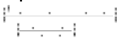
ticles distribution, equation,
P(n )
can be calculated from the following
ual neurons (processing elements), connections (topology), and a learning algorithm. The processing element calculates![]()
P(n )
![]()
![]()
3
( ) k 1 C
2a(n
1) 2
2b(n
1) 2 k 1
(2an 2
2bn ) k 1
the neuron transfer function of the summation of weighted
k 0 Q
C 1 ln
2a(n
1) 2
2an 2
k 1
2b(n 1)
2bn
(10)![]()
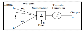
inputs. A simple neuron structure is shown in the fig 2. The neuron transfer function, f , is typically step or sigmoid func- tion that produces a scalar output ( n ) as in Eq. (15).
We assume a binomial and Poisson distributions for the prob-![]()
n ![]() f i wi Ii b
f i wi Ii b
(15)
ability distribution for the creation of charged pion pairs from
Where I i , wi
, b are the i th input, the i th weight and b the
one fireball of the forms,
1) Binomial Distribution of the form,
bias respectively.
A network consists of one or more layers of neurons. A![]()
(n2 )
![]()
![]()
N! p n2 q( N n2 )
(11)
layer of neurons is a number of parallel neurons. These layers
2) Poisson Distri
n2!( N f n2 )! form,
are configured in a highly interconnected topology.
bution on
the
(n2 )
![]()
![]()
![]()
2
p n2 e Np
(12)
n2 !
IJSER © 2012
International Journal of Scientific & Engineering Research Volume 3, Issue 3, March-2012 3
ISSN 2229-5518
The transfer function where chosen to be a tansigmoid func- tion for the hidden layer and a pureline function for the out- put
“Figure 2. Neuron model”
Neural network can be trained to perform a particular function by adjusting the values of the connections (weights) between elements. Training in simple is to make a particular input leads to a specific target output. The weights are ad- justed, based on a comparison of the output and the target, until the network output matches the target. Typically many such input/target pairs are used, in this supervised learning, to train a network.
The proposed ANNs in this paper was trained using Le-
“Figure 3. Comparison between the experimental and simulated
venberg–Marquardt optimization technique. This optimiza-
multiplicity distribution of pions
P(nch )
for p
n collisions at a)
tion technique is more powerful than the conventional gra-
50, b) 80 GeV/c and p
n collisions at, c) 100, d) 200 GeV/c:
dient descent techniques [31-35].
The Levenberg–Marquardt updates the network weights using the following rule:
(—) NN model, (……) PTFM model, (O) experimental data”.
![]()
![]()
W (J T J
![]()
I ) 1 J T e
Where J is the Jacobian matrix of derivatives of each error with respect to each weight, ![]() is a scalar, changed adaptively by the algorithm and e is an error vector.
is a scalar, changed adaptively by the algorithm and e is an error vector.
The only requirement for this method is a considerably
large memory for large problems. The initial training weights
were also chosen using the Nguyen–Widrow random genera-
tor in order to speed up the training process [31-35].
The charged particles multiplicity distributions using
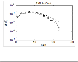
“Figure 4. Comparison between the experimental and predicted
PTFM, Eq. (14), are calculated for p![]()
n and p
![]()
n assuming ε
multiplicity distribution of pions
P(nch ) for p
n collisions at 400
given by![]()
![]()
an b
Where, a = 0.01, b = 0.35 for p![]()
n and a =
GeV/c: (—) NN model, (……) PTFM model, (O) experimental
0.01, b = 0.44 for p![]()
n . The results of these calculations are
data”.
represented in fig 1. a, b, c, d and e along with the experimen- tal data [27-30] which show fair agreement with the corres- ponding experimental data. It can be seen from fig 1. that the
layer, the trained NN model shows almost exact fitting. It
is worth mentioning that the NN training data did not include
emission of secondary particles is assumed to follow a bi-
the experimental data at PL![]()
400 GeV/c. This means that the
nomial distribution.
We have also modified our calculations using ANN model
and these calculations are represented in fig 3. a, b, c, d and fig
4. along with the same experimental data [27-30]. We have
also found some considerably variations in comparison with
fig 1.
Using the input-output arrangement, different network configurations were tried to achieve good mean squared error (MSE) and good performance for the network. It consists of an input layer (PLab , nch ), one hidden layers of 10 neurons, respec- tively, and an output layer consisting of one neuron P(nch ) .
NN model, not only simulated the trained fig 3. observations but also predicted the multiplicity distribution of charged pions for untrained observations as shown in fig 4. Then, the ANN technique is able to exactly model for multiplicity distri- bution at lab momenta for different beams in hadrons colli- sions.
Where net is 2-10-1 (input-i-j-k-output) and the equation is
p(nch ) = [(net: LWi (tansigmoid (pureline (net: I A + net: bi) +
net: b))))]
IJSER © 2012
International Journal of Scientific & Engineering Research Volume 3, Issue 3, March-2012 4
ISSN 2229-5518
Where, A is the input consists of two elements, net: I: linked weights between the input layer and 1st hidden layer, net: LW: linked weights bet. 3rd input layer and output layer, net: bi: biases for the hidden layer, net: b: biases for output layer.
I (input, hidden) (2, 10) =
4.7630 3.4592 -3.6549 -2.5606 4.0100
-2.9577 -0.1847 2.3966 3.3804 4.0002
-0.4856 | -1.8749 | 3.8754 | -1.7683 | 1.9219 |
-3.8578 | -4.8338 | 0.6290 | 1.9331 | 0.0420 |
LW (hidden, output) (10,1) = b (10,1) =
0.4117 -3.9147
0.2625 -3.5424
0.1937 1.9821
0.5731 3.0480
-0.0846 -0.2501
0.0104 -1.0340
-0.2503 0.2278
-2.6346 1.7418
0.8085 2.5888
-2.4237 -3.7691
[1] R. P. Feynman, Photon-Hadron Interactions (Reading, Mass: Benja- min) (1972)
[2] E. Fermi, Prog. Theor. Phys., 5,570 (1951), Phys. Rev., 81,683 (1950)
[3] J. Ranft, Phys. Lett., 31B, 529 (1970)
[4] Y. Nambo, the confinement of quarks. Sci. Am., 48 (1976)
[5] Cai-Xu and Chao W-q Meng T-C, phys. Rev., D 1986, 33, 1287 (1986)
[6] M. Jacob and R. Slansky, Phys. Rev., D 5, 1847 (1972)
[7] R. Hwa, Phys. Rev., D 1, 1790 (1970), Phys. Rev. Lett., 26, 1143 (1971)
[8] E. Fermi, Prog. Theor. Phys., 5, 568 (1950)
[9] P. Carruthers and C. Shih, Int. J. MOD. Phys, A 2, 1547 (1987)
[10] Z. Koba, H. B. Nielson and P. Olesen, Nucl. Phys., B40, 317 (1972)
[11] Al. Golokhvastov, Sov. J. Nucl. Phys., 27,430(1978), Sov.J.Nucl.Phys.,
30,128 (1979). Ina Sarcevic, Acta Physica Polonica, B19 (1988)
[12] P. Carruthers and C.C .Shih, Phys. Lett., 137B, l425 (1984)
[13] R. Hagedron, Nuovo Cim. Suppl. 1965, 3,147 (1965), Nuovo Cim. Suppl.,
1968, 6, 311 (1968), Nuovo Cim. Suppl., 1968, 6,311(1968), Nuovo Cim.
56A, 1027(1968), Nuovo Cim., 56A, 1027(1968), Nucl Phys., B 24, 93(1970), Nucl. Phys., B 24, 93(1970), J. Ranft, Ref. TH/851- CERN (1967), Ref. TH.1027-CERN (1969)
[14] GN Fowler, Phys. Rev. Lett., 57, 2119 (1986)
[15] A. Giovannini and L. Van Hove, Z Phys., C 30, 391(1986), P-K Mack- own and AW. Wolfendale, Proc Phys Soc Lond, 89,553(1966), N. Suzuki, Prog. Theor. Phys., 51, 1625(1974)
[16] T. T. Chou and C.N. Yang, Phys. Rev., D32, 1692(1985)
[17] B. Anderson, Phys. Rep., 97, 32 (1983), A. Capella, U. Sukhatme, Phys.
Rep. 236, 225 (1994)
[18] J. D. Bjokren, Phys. Rev., D27, 140(1983), L. Mclerran, Rev. Mod.Phys., 58,
1021(1986)
[19] H. van Hees, R. Rapp, Phys. Rev. C71, 034907 (2005), URL http://arxiv.org/abs/nucl- th/0412015, Su Houng Lee and Kenji Mo- rita, Pramana journal of physics, 72, 1, pp. 97-108(2009)
[20] AK Hamid, Can. J. Phys. 7, 76 (1998)
[21] P. Bhat, Using neural networks to identify jets in hadron–hadron colli- sions. Proceedings of The 1990 Summer Study on HEP, (1990), Re- search Directions––the Decade, Snowmass, Colorado
[22] RP. Lippman, IEEE Acoust Speech Signal Process Mag. (1987)
[23] M. Tantawy, M. El-Mashad, S. Gamiel and M. S. El- Nagdy, Chaos, Solitons and Fractals, 13, 919 (2002)
[24] M. Tantawy, M. El-Mashad, M.Y. El-Bakry, Indian J. Phys., 72A,
110(1998)
[25] M. Y. El-Bakry, 6th Conference on Nuclear and Particle Physics, (2007) November 17-21; Luxor, Egypt
[26] M. Tantawy, Ph.D. Dissertation (Rajasthan University, Jaipur, India)
(1980)
[27] J. E. A. Lys, C. T. Murphy, and M. Binkley, Phys. Rev. D 16, pp. 3127-
3136 (1977)
[28] T. Dombeck, L. G. Hyman, et al., Phys. Rev. D 18, pp. 86-91(1978)
[29] S. Dado, S .J. Barish, A. Engler, and R. W. Kraemer, Phys. Rev., D
;Vol/Issue20:7 (1979), D. K. Bhattacharjee, Phys. Rev., D 41, 9 (1990)
[30] Fermilab Proposal No.422 Scientific Spokesman: A. Fridman Centre De Recherches Nucleaires de Strasbourg Groupe des Chambres a Bulles a Hydrogene, France (1975)
[31] M.T. Hagan, Menhaj M.B, IEEE Trans Neural Networks 6:861–7 (1994)
[32] El-Sayed El-dahshan, A. Radi. Cent. Eur. J. Phys. 9(3), 874-883 (2011)
[33] S. Y. El-Bakry, El-Sayed El-dahshan, M. Y. El-Bakry. Ind. J. Phys., 85 (9),
1405-1413 (2011)
[34] S. Y. El-Bakry, El-Sayed El-dahshan, S. Al-Awfi and M. Y. El-Bakry.
ILNouvo Cimento, 125B (10), (2010)
[35] El-Sayed El-dahshan, A. Radi and M. Y. El-Bakry. Int. J. Mod. Phys. C,
20(11), 1817-825 (2009)
IJSER © 2012