International Journal of Scientific & Engineering Research, Volume 5, Issue 4, April-2014 20

ISSN 2229-5518

Application of Geomorphic Direct Runoff

Hydrograph Model for Arid Regions

Muhammad Shafqat Mehboob , Abdul Razzaq Ghumman, Hashim Nisar Hashmi, Abdul Rehman , Zafar M. A.

Abstract—Rainfall runoff models play a significant role in water resource engineering for future planning, management and development. This paper investigates the results obtained from two hydrologic techniques namely Nash Geomorphic Instantaneous Unit Hydrograph (GIUH) Model. Predictions are made for future use of Small Dams Organization Rawalpindi Division, Pakistan. Shahpur dam catchment was used as study area. Geomorphic parameters of Clark model were calculated using digital elevation model (DEM). Satellite imageries of catchment were processed using ArcGIS to estimate geomorphologic parameters. The model was applied for different storm events. Excess rainfall hyetograph was obtained from measured precipitation and direct surface runoff hydrograph was obtained by GIUH model. To check model efficiently two types of statistical parameters were used namely percentage error in peak (PEP) and percentage efficiency. The results from Nash GIUH were compared with those simulated by original Nash model and found that GIUH models are equally good even if the Nash model parameters are obtained by optimization.

Index Terms—Geomorphic, Model, PEP, Hydrograph, Events, Storms, Rainfall

1 INTRODUCTION

Water resource engineering is very old engineering as water is life. Water resource engineering projects are being given high importance word-wide. With population growth and development, the competition for water among agricultural, urban, industrial and environmental uses is increasing (Dawadi and Ahmad, 2013; Qaiser et al., 2013; Wu et al., 2013). Climate variability is resulting into extreme hydrologic events such as flash floods and hill torrents in some areas and drought in others, (Forsee and Ahmad, 2011; Ghumman et al. 2011, Ghumman et al. 2013 ). Water management can be improved by enhancing precipitation estimates (Kalra and Ahmad, 2012), flow estimates, sediment management, reservoir and deliver y infrastructure operation, conservation, maintenance; and governing institutions ((Carrier et al., 2013; Kalra et al., 2013a; Kalra et al., 2013b; Kalra et al., 2013c); Mirchi et al., 2012).
The engineering related to rainfall and runoff is highly complex because of the unpredictability of hydrological processes and global climate change (Mikhailova et al. 2012, Yasinskii and Kashutina 2012) and Dobrovolski (2012) have noticed prospective impact of global climate changes on river runoff. In present scenario of global changes substantial adaptation is required to guarantee appropriate engineering, planning and management of water resources. Readily available runoff simulations are utmost important for this purpose. At the same time runoff prediction from a catchment is very complicated and is difficult to simulate accurately.
It is further aggravated in case of catchments lying in arid or semiarid regions such as Shah Pur Dam in Attock District,

————————————————

Author

spatial variability and short interval run offs in arid and semi- arid regions. Mostly the relevant rainfall runoff data is scanty in these circumstances due to which the rainfall-runoff models hardly simulate the real response of the watershed. Identification of model parameters for arid and semi arid regions is a big issue due to smaller number of rainfall runoff events as compared to those in humid regions. It is utmost important to explore new tools as well as to investigate application of the existing tools for solving problems related to the real life in developing countries like Pakistan. Developing countries need to take help from the work done by the researchers world-wide. Nguyen et al. (2009) have modeled the Can Le catchment (Vietnam) runoff with the help of the geomorphologic instantaneous unit hydrograph (GIUH). Ahmad et al. (2009), Ahmad et al. (2010), Ghumman et al. (2011) and Ghumman et al. (2012) has presented work using one of Clark, Nash or GIUH models. Troitskaya et al., (2012) have developed new tools related to satellite altimetry for investigating water resources. Design of hydraulic structures, river improvement works, run off mitigation schemes, run off estimation, management of water resources and sustainable water resources planning and development preferably require work on application of the existing rainfall runoff models to simulate runoff. The work of Johnston and Kummu (2012) and Ahmed (2012) is important regarding this field. Ghumman et al., (2014) has done work on GIUH models for a large catchment. Although the floods in large catchment areas may be dangerous but the peaks of flash floods and hill torrents from small catchment areas are high and time to peak is small. Such floods may be more dangerous. Hence investigations regarding runoff simulations by GIUH rainfall runoff models for small areas in developing countries should also be given high importance. The

• Muhammad Shafqat Mehboob , MSc Scholor, University of Engineering and present paper deals with runoff simultaneous by application of

Technology Taxila,Pakistan PH-+923338219778. E-mail:

msmce102@yahoo.com

•

Co-Author

• Abdul Razzaq Ghumman, Professor, University of Engineering and Technology Taxila,Pakistan PH-+92519047638. E-mail: abdul.razzaq@uettaxila.edu.pk

Pakistan. There are usually intense rainfall events having high
two models for real life data of a small watershed in semi arid region of Pakistan having hill torrents and flash floods.

2 STUDY AREA

Shahpur Dam is a component of main small dam’s chain in
Punjab Barani Areas. The dam site is about 8 km north of

IJSER © 2014 http://www.ijser.org

International Journal of Scientific & Engineering Research, Volume 5, Issue 4, April-2014 21

ISSN 2229-5518

Fatehjang town District Attock. The dam site is situated in Kala
Chitta Range in Attock Distrcit, at about 50 km away from

RA 0.48 LΩ

Islamabad and 10 km from Fatehjang, District Attock. The topography of the area includs the area ranging from reduced

k = 0.7 � �

RBRL

� � (3)

V

level (RL) 424 to 540 m. The total catchment area is about 202 km2. The dam is of concrete gravity type and capacity of the spillway is 35600 ft3/s. The dam was commissioned by Small Dams Organization, Government of Punjab in 1982 and was completed in 1986 at a cost of Pakistani Rupees 36.5 million (about 1 million US $ according to the currency rate at that time).

3 MATERIALS AND METHODS

Where RA, RB , RL are Horton’s ratios, LΩ is length of highest order stream in kilometers and V is expected peak velocity in meters per second. k is in hours.

5 MODEL PERFORMANCE CHECK

To check efficiency of the models two error functions have been
used as given below.

5.1 Model efficiency

∑n (Qoi −Qsi )2

EFF = �1 −

i=n

� × 100 (4)

3.1 Estimation of Geomorphologic Parameters Geomorphologic characteristics of the Shahpur watershed were estimated using Arc GIS 10.1 software. The satellite imageries of Shahpur catchment was digitized and catchment area, stream order, stream areas and stream lengths were calculated. The maximum order of the streams in Shahpur dam watershed was 5. The corresponding length and area of the surface runoff of each channel order was measured. Using Horton’s law

∑n (Qoi −Q� oi)2

i=n

Here EFF is the percentage efficiency of the model, Qoi is the observed discharge of ith ordinate and Qsi is simulated discharge of ith ordinate. And ‘n’ is the total no of ordinates.

5.2 Percentage error in peak

Qps

geomorphologic parameters, such as bifurcation ratio (RB),
stream length ratio (RL), and stream area ratio (RA), were calculated for the each order channels.
Qpep = �1 −

Qpo

� × 100 (5)

4 NASH AND GIUH-NASH MODELS

The original Nash’s model is based on linear reservoir theory for
input and output in a watershed. The ordinates of Nash’s
Instantaneous Unit Hydrograph are given as Nash (1958)
Where Qpep is percentage error in discharge in ft3/s. Qps is the
calculated peak discharge and Qpo is the observed peak discharge in ft3/s. Similarly errors can be found in time to peak (PETp) and volume of runoff (PEV).

6 SUMMARY, RESULTS AND DISCUSSIONS

The parameters of Nash GIUH model (n and k) are calculated
from the geomorphic characteristic of the watershed area where
Un(t) = �

� �t n−1 e−t

(1)
as the original Nash model parameters were determined by hit and trial optimization. The model was applied to four rainfall

k

k Γ (n) k

Where ‘n’ and ‘k’ are parameters obtained from geomorphic characteristics of the catchment and‘t’ is the time and Γ(n)=(n-1)! for integer n. Nash’s proposed equation is two parameter gamma function. The first parameter ‘n’ is the shape factor or degrees of freedom (number of linear cascades attenuating the IUH peak) and second parameter ‘k’ is the scale factor (time of storage, equal for all linear cascades).The

parameters n and k are related as � t � = n − 1

k

So the right hand side (RHS) of equation of above equation can
be written as
events of 2013 and simulated runoff was compared with
observed direct runoff hydrographs. The peak velocity was calculated using the equations mentioned above and time of concentration was obtained from geomorphic parameters. The kinematic wave coefficient was estimated to be 0.7 (s−1.m−1/3). The length of longest stream was 23.47 km. The parameter values of both the models are given in table 2. It is observed that he parameters estimated from geomorphic characteristics are close to the best parameters calculated by hit and trial for Nash model. The runoff generated by the two models for different events is shown in Figs. 1 to 10. The model efficiency and the error between the observed and simulated peak runoff (QPEP),

�(n−1) � e1−n = 0.58 �RB�

0.55

R0.05

time to peak (PETp) and volume of runoff (PEV) is given in table 3. It is observed that results of both the models Nash and

Γ (n)

RA L

(2)
Nash GIUH are very close. This shows that in case the data is
Rosso (1984) proposed expressions using regression analysis for estimation of Nash’s model parameter ‘n’ and ‘k’ as:
scanty and calibration/validation of the runoff model is not possible then the GIUH model can be used. The efficiency of GIUH model ranges from 44% to 99%. In Nash GIUH model
RB
n = 3.29 �
RA

0.78

�

0.07

L

storm event 2 is most efficient. Same is the case with time to
reach the peak discharge.

IJSER © 2014 http://www.ijser.org

International Journal of Scientific & Engineering Research, Volume 5, Issue 4, April-2014 22

ISSN 2229-5518

Table 1: Geomorphologic parameters and stream order for Shahpur catchment.

Table 2: Nash and Nash GIUH model parameters

Table 3:Nash and Nash GIUH model’s parameters

IJSER © 2014 http://www.ijser.org

International Journal of Scientific & Engineering Research, Volume 5, Issue 4, April-2014 23

ISSN 2229-5518

1800.00

1600.00

1400.00

1200.00

800.00

600.00

400.00

200.00

0.00

Nash observed Nash GIUH

0 5 10 15 20 25 30 35 40

Time (hours)

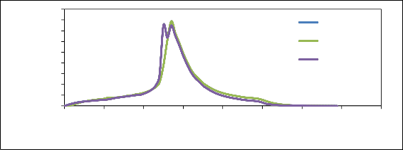
Fig. 1:The Calculated DSRO hydrographs at outlet by the Nash , Clark, Nash GIUH and Clark GIUH models, and observed outlet
DSRO hydrograph for Event No.1

80.00

70.00

60.00

50.00

40.00

30.00

20.00

10.00

0.00

Nash observed Nash (GIUH)

1 3 5 7 9 11 13 15 17

Time (hours)

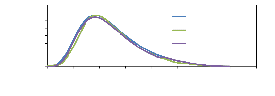
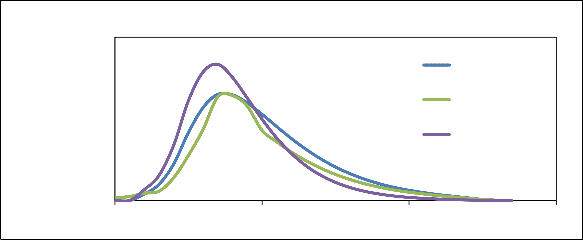
Fig. 2:The Calculated DSRO hydrographs at outlet by the Nash , Clark, Nash GIUH and Clark GIUH models, and observed outlet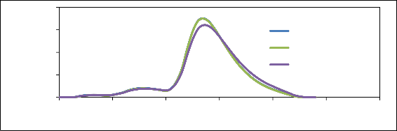

DSRO hydrograph for Event No.2

400.00

300.00

200.00

100.00

nash observed Nash GIUH

0.00

0 5 10 15 20 25 30

Time (hours)
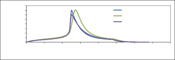
Fig. 3:The Calculated DSRO hydrographs at outlet by the Nash , Clark, Nash GIUH and Clark GIUH models, and observed outlet
DSRO hydrograph for Event No.3

IJSER © 2014 http://www.ijser.org

International Journal of Scientific & Engineering Research, Volume 5, Issue 4, April-2014 24

ISSN 2229-5518

60.00

50.00

30.00

20.00

10.00

0.00

nash observed Nash GIUH

0 5 10 15 20 25 30

Time (hours)

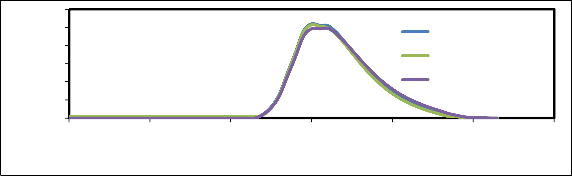
Fig. 4:The Calculated DSRO hydrographs at outlet by the Nash , Clark, Nash GIUH and Clark GIUH models, and observed outlet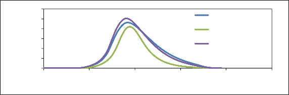

DSRO hydrograph for Event No.4

500.00

400.00

nash

observed

200.00

100.00

0.00

Nash GIUH

0 5 10 15 20 25

Time (hours)

Fig. 5:The Calculated DSRO hydrographs at outlet by the Nash , Clark, Nash GIUH and Clark GIUH models, and observed outlet
DSRO hydrograph for Event No.5

600.00

500.00

400.00

nash observed

200.00

100.00

0.00

Nash GIUH

0 5 10 15 20 25

Time (hours)

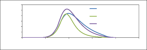
Fig. 6:The Calculated DSRO hydrographs at outlet by the Nash , Clark, Nash GIUH and Clark GIUH models, and observed outlet
DSRO hydrograph for Event No.6

IJSER © 2014 http://www.ijser.org

International Journal of Scientific & Engineering Research, Volume 5, Issue 4, April-2014 25

ISSN 2229-5518

1600.00

1400.00

1200.00

1000.00

800.00

600.00

400.00

200.00

0.00

nash

observed

Nash GIUH

0 5 10 15 20 25 30 35 40

Time (hours)

Fig. 7:The Calculated DSRO hydrographs at outlet by the Nash , Clark, Nash GIUH and Clark GIUH models, and observed outlet
DSRO hydrograph for Event No.7

300.00

200.00

100.00

0.00

nash observed Nash GIUH

0 5 10 15 20 25 30

Time (hours)

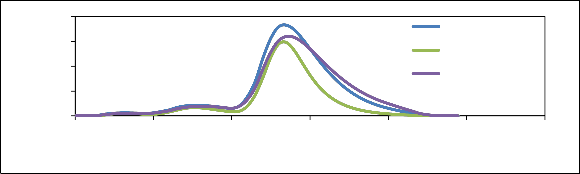
Fig. 8: The Calculated DSRO hydrographs at outlet by the Nash, Clark, Nash GIUH and Clark GIUH models, and observed outlet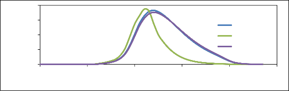

DSRO hydrograph for Event No.8.

800.00

400.00

200.00

nash observed Nash GIUH

0.00

0 5 10 15 20 25

Time (hours)

Fig. 9: The Calculated DSRO hydrographs at outlet by the Nash , Clark, Nash GIUH and Clark GIUH models, and observed outlet
DSRO hydrograph for Event No.9

IJSER © 2014 http://www.ijser.org

International Journal of Scientific & Engineering Research, Volume 5, Issue 4, April-2014 26

ISSN 2229-5518

40.00

30.00

20.00

10.00

nash observed Nash(GIUH)

0.00

10 15 20 25

Time (hours)

Fig. 10: The Calculated DSRO hydrographs at outlet by the Nash , Clark, Nash GIUH and Clark GIUH models, and observed outlet
DSRO hydrograph for Event No.10
Table 03: EFF and PEP of the Nash and Nash GIUH models for 10 storm events.

7 CONCLUSION

From the results obtained it is concluded that Nash-GIUH model gives equally good results as compared to the original Nash model. In Nash GIUH model efficiency of the model ranges from 96% to 44% in first six events. The next four events have efficiency of more than 70% which means that the model is efficient and can be applied to any rainfall runoff event. In case
of % error in peak discharge this error ranges from -38% to 21% which means that there is variation but in case of next four events mostly a lower value of error in peak discharge is obtained.

REFERENCES

[1] Dobrovolski S. G., (2012), “Year to Year and many year runoff variations in World Rivers”, Water Resources, Vol.
38, No. 6, pp. 693–708.
[2] Dzhamalov R. G., Krichevets G. N., and Safronova T. I., (2012), “Current changes in water resources in Lena River Basin, Water Resources, Vol. 39, No. 2, pp. 147–160.
[3] Dawadi S, Ahmad S., (2013). “Evaluating the impact of
Demand-Side Management on water resources under changing climatic conditions and increasing population”, Journal of Environmental Management, 114, 261-275. DOI:
10.1016/j.jenvman.2012.10.015.
[4] Ghumman A. R., Ahmad M. M., Hashmi H. N., and Kamal M. A., (2011), “Regionalization of Hydrologic Parameters of Nash Model”, Water Resources, Vol. 38, No. 6, pp.
735–744.
[5] Ghumman A. R., Ahmad M. M., Hashmi H. N., Kamal M.
A. (2012), “Development of geomorphologic instantaneous unit hydrograph for a large watershed”,

Environmental Monitoring and Assessment, Volume 184,

Issue 5, pp 3153-3163.
[6] Ghumman A. R., Khan QU, Hashmi H. N., Ahmad M. M., (2014), “Comparison of Clark, Nash and Geographical

IJSER © 2014 http://www.ijser.org

International Journal of Scientific & Engineering Research, Volume 5, Issue 4, April-2014 27

ISSN 2229-5518

Instantaneous unit hydrograph models for arid and semi arid regions, Water Resources, Vol 41.
[7] Kalra A, Ahmad S. (2012). “Estimating annual precipitation for the Colorado River Basin using oceanic-
atmospheric oscillations”, Water Resources Research, 48: W06527. DOI:10.1029/2011WR010667.
[8] Kalra A, Ahmad S, Nayak A. (2013a), “Increasing streamflow forecast lead time for snowmelt driven
catchment based on large scale climate patterns”,

Advances in Water Resources 53: 150-162.

[9] Kalra A, Li L, Li X, Ahmad S. (2013b), “Improving streamflow forecast lead time using oceanic-atmospheric
oscillations for Kaidu river basin, Xinjiang, China”, ASCE Journal of Hydrologic Engineering18 (8): 1031-1040. doi:
10.1061/(ASCE)HE.1943-5584.0000707.
[10] Kalra A, Miller WP, Lamb KW, Ahmad S, Piechota T. (2013c). “Using large scale climatic patterns for improving long lead time streamflow forecasts for Gunnison and San Juan River Basins”, Hydrological Processes 27 (11): 1543-1559.
[11] Mikhailova M. V., Mikhailov V. N., and Morozov V.
N., (2012), “Extreme hydrological events in the Danube
River Basin over the last decades”, Water Resources, vol. 39, No. 2, pp. 161–179.
[12] Mirchi A, Kaveh M, Watkins D, Ahmad S. (2012), “Synthesis of system dynamics tools for holistic conceptualization of water resources problems”, Water

Resources Management 26(9): 2421-

2442.DOI:10.1007/s11269-012-0024-2.
[13] Nguyen H. Q., Maathuis B. H.P., Rientjes T. H.M., (2009), “Catchment storm runoff modelling using the geomorphologic instantaneous unit hydrograph”, Geocarto International, 24:5, 357-375
[14] Qaiser K, Ahmad S, Johnson W, Batista J. (2013), “Evaluating water conservation and reuse policies using ayynamic water balance model”, Environmental Management, 51(2): 449-458. DOI: 10.1007/s00267-
012-9965-8.
[15] Troitskaya Yu. I., Rybushkina G. V., Soustova I. A., Balandina G. N., Lebedev S. A., Kostyanoi A. G., Panyutin A. A., Filina L. V., (2012), “Satellite altimetry of inland water bodies”, Water Resources, vol. 39, no.
2, pp. 184–199.
[16] Wu G, Li L, Ahmad S, Chen X, and Pan X (2013), “A
dynamic model for vulnerability assessment of regional water resources in arid areas, A case study of Bayingolin, China, Water Resources Management 27(8):3085-3101. DOI: 10.1007/s11269-013-0334-z.
[17] Yasinskii S. V. and Kashutina E. A., (2012), “Effect of regional climate variations and economic activity on
changes in the hydrological regime of watersheds and small-river runoff”, Water Resources, vol. 39, No. 3, pp. 272–293.

IJSER © 2014 http://www.ijser.org