International Journal of Scientific & Engineering Research, Volume 4, Issue 6, June-2013 1659
ISSN 2229-5518
Analysis of the k-є and k-ω standard models for
the simulation of the flow over a National
Advisory Committee for Aeronautics (NACA)
4412 airfoil
Amit Saraf, Farook Ahmed Nazar, Sushil Pratap Singh
Abstract-The analysis of the two dimensional subsonic flow over a National Advisory Committee for Aeronautics (NACA) 4412 airfoil at various angles of attack and operating at a velocity of 50 m/s is presented. The flow was obtained by solving the steady-state governing equations of continuity and momentum conservation combined with any two turbulence models [k-є standard and k-ω standard] aiming to the validation of these models through the comparison of the predictions and the free field experimental measurements for the selected airfoil. The aim of the work was to find out the optimum turbulent model out of two models b y showing the behavior of the airfoil at specified conditions and to establish a verified solution method. Dependence of the drag CD and lift coefficient CL on the angle of attack was determined using two different turbulence models. Turbulent flows are significantly affected by the presence of walls, where the viscosity affected regions have large gradients in the solution variables and accurate presentation of the near wall region determines successful prediction of wall bounded turbulent flows. In this paper coefficient of lift from software is compared with published practical data. Calculations were done for constant air velocity altering only the angle of attack for every turbulence model tested. This work highlighted two areas in computational fluid dynamics (CFD) that require further investigation: transition point prediction and turbulence modeling. In this work calculations shows that the turbulence models used in commercial CFD codes does not give yet accurate results at high angles of attack.
Keywords: - Airfoil; Angle of attack; coefficient of drag; coefficient of lift; computational fluid dynamics; Fluid-Flow; Turbulent.
1 INTRODUCTION
—————————— ——————————
order to validate the present simulation
The first step in modeling a problem involves the
N fluid dynamics, turbulence or turbulent flow is a fluid regime characterized by chaotic, stochastic property changes. This includes low momentum diffusion, high momentum convection and rapid variation of pressure and velocity in space and time. In this analysis, the Standard k-є model and the Standard k-ω model were combined with the governing equations for the numerical solution of the flow field over the NACA 4412 airfoil and existing experimental data from reliable sources Abbott et al.,
1959[1] are performed to validate the computational results. In order to include the transition effects in the aerodynamic coefficients calculation and get accurate results for the drag coefficient, a new method was used. In this work, the NACA 4412, the well documented airfoil from the4-digit series of NACA airfoils, is utilized. NACA 4412 airfoil has a maximum thickness of 12% with a camber of 4% located
40% back from the airfoil leading edge (or 0.4c). Velocity for the simulations was 50m/s, same with the reliable experimental data from Abbott and Von Doenhoff (1959), in
————————————————
• Amit Saraf is persuing Mtech from Rajasthan Technical University Kota, Rajasthan, India phone: +91-9928396705; e-mail: amitsaraf11@rediffmail.com
• Farooq Ahmad Najar is research scholar with the department of
Mechanical Engineering National Institute of Technology
Shrinagar,India phone: +91-9797702635; e-mail: frq.engr@gmail.com
• Sushil Pratap Singh with the Mechanical Engineering Department, Bhartiya Institute of Engineering & Technology, Sikar Rajasthan,India
phone:+91-9983956818-e-mail: sp911@rediffmail.com
creation of the geometry and the meshes with a preprocessor. The majority of time spent on a CFD project in the industry is usually devoted to successfully generating a mesh for the domain geometry that allows a compromise between desired accuracy and solution cost. After the creation of the grid, a solver is able to solve the governing equations of the problem. The basic procedural steps for the solution of the problem are the following. First, the modeling goals have to be defined and the model geometry and grid are created. Then, the solver and the physical models are stepped up in order to compute and monitor the solution. Afterwards, the results are examined and saved and if it is necessary we consider revisions to the numerical or physical model parameters.
In this project, curves for the lift and drag characteristics of
the NACA 4412 airfoil were developed. This airfoil was
chosen because it has been used in many constructions.
Typical examples of such use of the airfoil are the B-19
Flying Fortress and Cessna 142, the helicopter Sikorsky S-65
SH-4 Sea King as well as horizontal and vertical axis wind
turbines.
According to Nathan Logsdon [2] both a 2-D and 3-D
model of the four-digit airfoil 0012 were created. When
these models were run in FLUENT under the same
conditions identical results were produced. This goes to
prove the validity of using a simpler 2-D model for analyzing airflow over airfoils instead of the more time consuming 3-D model.
IJSER © 2013 http://www.ijser.org
International Journal of Scientific & Engineering Research, Volume 4, Issue 6, June-2013 1660
ISSN 2229-5518
2 MATHEMATICAL FORMULATION & TURBULENCE
MODELING
For all flows, the solver solves conservation equations for mass and momentum. Additional transport equations are
also solved when the flow is turbulent. The equation for
ω model in FLUENT is based on the Wilcox k-ω model
,which incorporates modifications for low-Reynolds-
number effects, compressibility, and shear flow spreading.
The turbulence kinetic energy, k, and the specific
dissipation rate, ω, are obtained from the following
transport equations

∂ ∂ ∂ ∂k
conservation of mass or continuity equation can be written as follows:


(ρk) + (ρkui ) = �
∂t ∂x ∂xi
� + Gk − Yk + Sk (7)
∂xi
𝑑𝜌 + ∇. (𝜌𝑢�⃗) = 𝑆
(1)


∂ (ρω) + ∂

∂ ∂ω � + G
− Y + S
(8)

𝑑𝑡 𝑚

(ρωui ) = �
∂t ∂x ∂xi
∂xi
ω ω ω
Equation 1 is the general form of the mass conservation
equation and is valid for incompressible as well as
compressible flows. The source Sm is the mass added to the
continuous phase from the dispersed second phase (for
example, due to vaporization of liquid droplets) and any user-defined sources. Conservation of momentum in an inertial reference frame is described by Equation 2

𝜕(ρ𝑢�⃗) + ∇. (ρ𝑢�⃗𝑢�⃗) = −∇𝑝 + ∇. (𝜏) + 𝜌𝑔⃗ + 𝐹⃗ (2)
𝜕𝑥
Where p is the static pressure, t is the stress tensor
(described below) and g�⃗ and F��⃗ are the gravitational body
force and external body forces (for example, that arise from
interaction with the dispersed phase), respectively. F��⃗ also
contains other model-dependent source terms such as
porous-media and user-defined sources. The stress tensor
t is given by:

τ� = µ �(∇u�⃗ + ∇u�⃗T ) − 2� ∇. �u⃗I (3)
3
Where µ is the molecular viscosity, I is the unit tensor, and
the second term on the right hand side is the effect of
In these equations, Gk represents the generation of turbulence kinetic energy due to mean velocity gradients. Gω represents the generation of ω. Γk and Γω represent the effective diffusivity of k and ω, respectively. Yk and Yω represent the dissipation of k and ω due to turbulence. All of the above terms are calculated as described below. Sk and Sω are user-defined source terms
2.2 k-є standard turbulence model
The k-є model is well described in the literature and has been widely used. This model was derived by assuming that the flow is fully turbulent and the effects of molecular viscosity are negligible. For locations near walls, the standard k-e model, therefore, demands an additional model,which comprises the effects of molecular viscosity. In this situation, wall functions based on semi-empirical formulas and functions are employed.
The turbulence kinetic energy, k and its rate of dissipation,
є are obtained from the following transport equations:
volume dilation. For the 2-D, steady and incompressible ∂ ∂
∂ µ ∂k
flow the continuity equation is:


∂u + ∂v = 0 (4)


(ρk) + (ρku ) = ��μ + t � � + G + G − ρϵ − Y + S (9)
∂t ∂xi ∂xj σk ∂xj
∂x ∂y
∂ ∂ ∂
µt ∂ϵ ϵ
Momentum equations for viscous flow in x and y


(ρϵ) + (ρϵu ) = ��μ + � � + C (G + C G ) −

∂t ∂x ∂x σ ∂x k
i j ϵ j
ϵ2
directions are, respectively


ρ Du = − ∂p + ∂τxx + ∂τyx + ρf
(5)
C2ϵ ρ
+ Sϵ (10)
Dt ∂x
∂x ∂y x
In these equations, Gk represents the generation of
turbulence kinetic energy due to the mean velocity
ρ Dv = − ∂p + ∂τxy + ∂τyy + ρf
(6)
gradients, Gb is the generation of turbulence kinetic energy


Dt ∂y
∂x ∂y x
due to buoyancy. YM represents the contribution of the
where due to characteristics of the 2-D flow in continuity
equation the term ∂w⁄∂z and in momentum equation,
fluctuating dilatation in compressible turbulence to the overall dissipation rate.
∂τzx�∂z
and
∂τzy� drop out. The continuity and
momentum equations are combined with one of the
following turbulence models which are briefly presented as
follows:
2.1 k-ω standard turbulence model
The standard k-ω model is one of the most common turbulence models. It includes two extra transport equations to represent the turbulent properties of the flow. The first transported variable is turbulent kinetic energy, k, similar to the turbulent kinetic energy equation of the standard k- є model. The second is the specific dissipation, ω, which can also be thought of as the ratio of e to k. The model incorporates modifications for low-Re effects, compressibility and shear flow spreading. The standard k-
3 COMPUTATIONAL METHOD
The free stream temperature is 300 K, which is the same as the environmental temperature. The density of the air at the given temperature is ρ=1.225 kg/m3 and the viscosity is
µ=1.7894×10⁻⁵kg/ms. for this velocity, the flow can be described as incompressible. This is an assumption close to reality and it is not necessary to resolve the energy equation. A segregated, implicit solver was utilized (Fluent
6.3.26, 2006) Calculations were done for angles of attack ranging from -18o to 18°. The airfoil profile, boundary conditions and meshes were all created in the pre-processor Gambit 2.3.16. The pre-processor is a program that can be employed to produce models in two and three dimensions, using structured or unstructured meshes, which can consist
IJSER © 2013 http://www.ijser.org
International Journal of Scientific & Engineering Research, Volume 4, Issue 6, June-2013 1661
ISSN 2229-5518
of a variety of elements, such as quadrilateral, triangular or tetrahedral elements. The resolution of the mesh was greater in regions where greater computational accuracy was needed, such as the region close to the airfoil. The first step in performing a CFD simulation should be to investigate the effect of the mesh size on the solution results. Generally, a numerical solution becomes more accurate as more nodes are used, but using additional nodes also increases the required computer memory and computational time. The appropriate number of nodes can be determined by increasing the number of nodes until the mesh is sufficiently fine so that further refinement does not change the results.
4 RESULTS AND DISCUSSION
4.1 Simulation Outcomes of Static Pressure
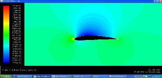
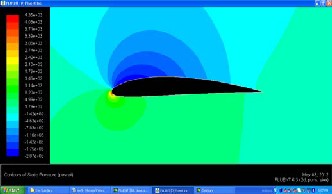
From the contour of pressure coefficient, we see that there is a region of high pressure at the leading edge (stagnation point) and region of low pressure on the upper surface of airfoil. This is of what we expected from analysis of velocity vector plot. From Bernoulli equation, we know that whenever there is high velocity, we have low pressure and vice versa. Figure 1 to 6 shows the simulation outcomes of static pressure at angles of attack 00 to15° with three used model. The pressure on the lower surface of the airfoil was greater than that of the incoming flow stream and as a result it effectively “pushed” the airfoil upward, normal to the incoming flow stream. On the other hand, the components of the pressure distribution parallel to the incoming flow stream tended to slow the velocity of the incoming flow relative to the airfoil, as do the viscous
stresses.
Fig1 Contours of static pressure at 0oangle of attack with k-є turbulent
model
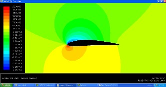
Fig. 2 Contours of static pressure at 9oangle of attack with k-є
turbulent model
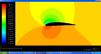
Fig.3 Contours of static pressure at 15oangle of attack with k-є
turbulent model
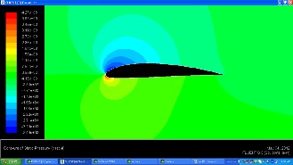
Fig.4 Contours of static pressure at 0oangle of attack with k-ω
turbulent model
Fig.5 Contours of static pressure at 9oangle of attack with k-ω
turbulent model
Fig. 6 Contours of static pressure at 15oangle of attack with k-ω
turbulent model
IJSER © 2013 http://www.ijser.org
International Journal of Scientific & Engineering Research, Volume 4, Issue 6, June-2013 1662
ISSN 2229-5518
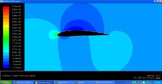
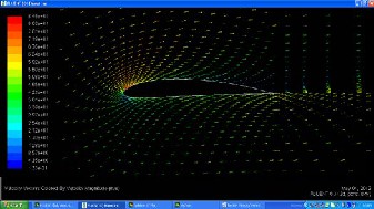
4.2 Contours of Velocity Component
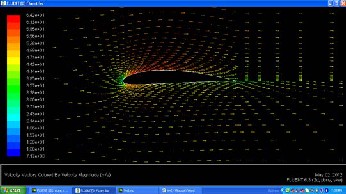
Contours of velocity components at angles of attack 3, 9 and 15° are also shown (Figures 7 to 9). The trailing edge stagnation point moved slightly forward on the airfoil at low angles of attack and it jumped rapidly to leading edge at stall angle. A stagnation point is a point in a flow field where the local velocity of the fluid is zero. The upper surface of the airfoil experienced a higher velocity compared to the lower surface. That was expected from the pressure distribution. As the angle of attack increased the upper surface velocity was much higher than the velocity of the lower surface. As can be seen, the velocity of the upper surface is faster than the velocity on the lower surface
Fig.7 Contours of velocity components at 0oangle of attack with k-ω
turbulent model
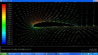
Fig.8 Contours of velocity components at 9oangle of attack with k-ω
turbulent model
Fig.9 Contours of velocity components at 15oangle of attack with k-ω
turbulent model.
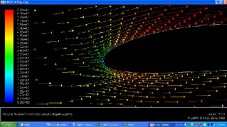
Fig.10 Contours of velocity components on leading edge
On the leading edge, we see a stagnation point where the velocity of the flow is nearly zero. The fluid accelerates on the upper surface as can be seen from the change in colors of the vectors. On the trailing edge, the flow on the upper surface decelerates and converges with the flow on the lower surface.
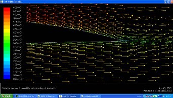
Fig.11 Contours of velocity components on trailing edge
4.3 Curves of Pressure Coefficient
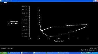
The lower curve is the upper surface of the airfoil and has a negative pressure coefficient as the pressure is lower than the reference pressure as shown in fig from 12 to 17
Fig.12 Pressure coefficient at 0oangle of attack with k-є turbulent
model
IJSER © 2013 http://www.ijser.org
International Journal of Scientific & Engineering Research, Volume 4, Issue 6, June-2013 1663
ISSN 2229-5518
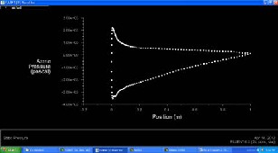
Fig.13 Pressure coefficient at 9oangle of attack with k-є turbulent
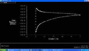
model
Fig.14 Pressure coefficient at 15oangle of attack with k-є turbulent
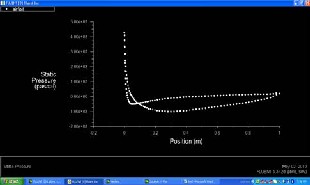
model
Fig.15 Pressure coefficient at 0oangle of attack with k-ω turbulent
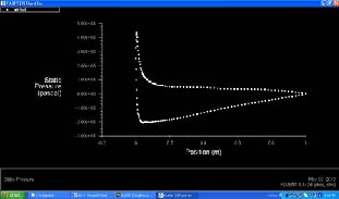
model
Fig.16 Pressure coefficient at 9oangle of attack with k-ω turbulent
model
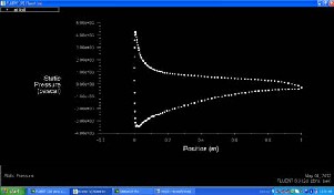
Fig.17 Pressure coefficient at 15oangle of attack with k-ω turbulent
model
4.4 Variation of CL with Angle of Attack
Simulations for various angles of attack were done in order to be able to compare the results from the different turbulence models and then validate them with existing experimental data from reliable sources Abbott[1]. To do so, the models were solved with a range of different angles of attack from -18 to 18°.On an airfoil, the resultants of the forces are usually resolved into two forces and one moment. The component of the net force acting normal to the incoming flow stream is known as the lift force and the component of the net force acting parallel to the incoming flow stream is known as the drag force. The curves of the lift and the drag coefficient are shown for various angles of attack, computed with three turbulence models and compared with experimental data. Fig. 18 and 19 shows variation of CL with angle of attack with three turbulent models.
Fig.18 variation of CL with angle of attack with k-ω turbulent models
IJSER © 2013 http://www.ijser.org
International Journal of Scientific & Engineering Research, Volume 4, Issue 6, June-2013 1664
ISSN 2229-5518
Fig.19 variation of CL with angle of attack with k-є turbulent models
5 DISCUSSIONS
Figure 20 shows that at low angles of attack, the dimensionless lift coefficient increased linearly with angle of attack. Flow was attached to the airfoil throughout this regime. At an angle of attack of roughly 14 to 15°, the flow on the upper surface of the airfoil began to separate and a condition known as stall began to develop. All three models had a good agreement with the experimental data at angles of attack from -10 to 10° and the same behavior at all angles of attack until stall. It was obvious that the k-ω and Spalart-Allmaras turbulence model had the approximately same behavior with the experimental data as well as after stall angle. Near stall, disagreement between the data was shown. The lift coefficient peaked
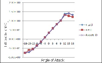
and the drag coefficient increased as stall increased.
Fig.20 Comparison between experimental data from Abott et al and three different turbulent models simulation result of the lift coefficient curve for NACA 4412 airfoil.
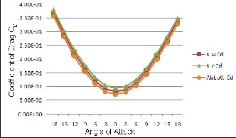
Fig.21 Comparison between experimental data from Abott et al and three different turbulent models simulation result of the Drag Coefficient curve for NACA 4412 airfoil
6 CONCLUSIONS
This paper showed the behavior of the 4-digit symmetric airfoil NACA 4412 at various angles of attack. The pressure on the lower surface of the airfoil was greater than that of the incoming flow stream and as a result it effectively “pushed” the airfoil upward, normal to the incoming flow stream. The trailing edge stagnation point moved slightly forward on the airfoil at low angles of attack and it jumped rapidly to leading edge at stall angle. A stagnation point is a point in a flow field where the local velocity of the fluid is zero. The upper surface of the airfoil experienced a higher velocity compared to the lower surface. That was expected from the pressure distribution. As the angle of attack increased the upper surface velocity was much higher than the velocity of the lower surface. The computational results from the three turbulence models were compared with experimental data where the boundary layer formed around the airfoil is fully turbulent and they agreed well. The most appropriate turbulence model for these simulations is the k-ω two-equation model, has a good agreement with the published experimental data Abbott [1] of other investigators for a wider range of angles of attack.
7 FUTURE WORKS
This study could be considered as an introductory study to illustrate the utility of computational flow analysis (CFD) in the analysis of airfoil with different turbulent models. Further and more complete studies are needed to apply it on 3-D geometry of airfoil.
Most important future Points are:
1) Mesh refinement (Grid independency) to get more reliable results. This is needed for applying a proper wall function to numerical computational model.
2) Different materials can be used for airfoil. Effect of material on lift coefficient could be studied.
3) Transition point could be changed and effect of this
could be studied.
4) Comparison of these used model and also other models
IJSER © 2013 http://www.ijser.org
International Journal of Scientific & Engineering Research, Volume 4, Issue 6, June-2013 1665
ISSN 2229-5518
could be used on various type of shape or series and result could be compared with experimental data.
REFERENCES
[1] G Abbott IH, Von Doenhoff AE. Theory of Wing Sections. ISBN 486-
60586-8Dover Publishing, New York. (1959).
[2] Nathan Logsdon. A PROCEDURE FOR NUMERICALLY ANALYZING AIRFOILS AND WING SECTIONS, University of Missouri, pp 2-53– Columbia (2006).
[3] Emrah KULUNK and Nadir YILMAZ, computer aided design and
performance analysis of HAWT Blades.IATS-09 may karabuk,turkey. vol
9 pp13-15 Aug2009.
[4] Douvi C. Eleni*, Tsavalos I. Athanasios and Margaris P. Dionissios
Evaluation of the turbulence models for the simulation of the flow over a
National Advisory Committee for Aeronautics (NACA) 0012 airfoil
,JMER vol 4(3)pp100-111March(2012).
[5] Russell Phillips DEVELOPMENT OF A RECIPROCATING AEROFOIL WIND ENERGY HARVESTER. , IATS-09 may karabuk,turkey. vol 9 pp405-422( December 2008 ).
[6] Badran O. Formulation of Two-Equation Turbulence Models for
Turbulent Flow over a NACA 4412 Airfoil at Angle of Attack 15 Degree,
6th International Colloquium on Bluff Bodies Aerodynamics and
Applications, Milano, vol 6 pp20-24 July. (2008).
[7] Ma L, Chen J, Du G, Cao R. Numerical simulation of aerodynamic performance for wind turbine airfoils. Taiyangneng Xuebao/Acta Energiae Solaris Sinica, vol 31: pp203-209. (December
2010).
[8] Bacha WA, Ghaly WS. Drag Prediction in Transitional Flow over Two-
Dimensional Airfoils, Proceedings of the 44th AIAA Aerospace Sciences
Meeting and Exhibit, Reno, NV.vol 44 pp45-53 (2006).
[9] M Ahmed Abd Almahmoud Ahmed Yassin Abubaker Mohammed Ahmed Elbashir, Simulation around airfoil NACA 4412, University of Khartoum, Rabi alawal 1432, pp1-19 (Feb2011).
[10] John D.Anderson,Jr, Fundamental of Aerodynamics, 3rd Edition, ISBN 0-
07-237335-0 McGraw-Hill Higher Education Publishing, New York.
(2001).
[11] S.M.Yaha,Fundamental of compressible flow,fourth edition,ISBN 978-81-
224-2668-7,New Age International Limited Publisher, India(2010).
[12] R Fluent6.3 Tutorial Guide, Copyright ©2006 by Fluent Inc, Fluent Inc.
Centerra Resource Park 10 Cavendish Court Lebanon, NH 03766, Sep
2006.
[13] Gambit2.2 Tutorial Guide, Copyright ©2006 by Fluent Inc, Fluent Inc.
Centerra Resource Park 10 Cavendish Court Lebanon, NH 03766, Sep
2004.
[14] G.Manikanadan M Ananda Rao. Effect of Maximum thickness location of an aerofoil on aerodynamic charecteristic. IJAEST vol 3 issue 2pp 122-
133(2011)
IJSER © 2013 http://www.ijser.org