Inte rnatio nal Jo urnal o f Sc ie ntific & Eng inee ring Re se arc h, Vo lume 2, Issue 12, Dece mbe r-2011 1

ISS N 2229-5518

Analysis of seismic waveforms using full-bridge voltage source inverter

Mehrdad Habibi Departement of Electrical Engineering Iran University of Science and Technolog y

(IUST)

Tehran, Iran

Abs tract - The current research talks about a designed accelerometer system w hich is able to measure every type of mechanical vibration. The applied vibration in this survey is called seismic w ave. Then the measured w ave by this novel system is transf ormed to a specif ic f unction using spline interpolation. This explicit f unction can be used as a ref erence signal in the technique PWM to be made in current f orm in such a w ay that it becomes exactly similar to the shape of vibration w ave caused by the inverter of tw o- branch, full-bridge voltage supply. The aim is eventually to use this approach f or some technical applications such as designing of an seismic table.

Ke ywor ds : s eis mic wave, acce lero meter, inverter, s pline interpolation, s imu lation

——————————  ——————————

1. Introduction

In electrical, mechanical or electro-mechanical equipment and instruments, the effects of energy-carrying waves that may be propagated in electrical or mechanical forms, should be precisely investigated whereas they often do not follow the behavior of standard waveform. Study and control of these waves due to their unpredictable and occasionally intense energy, may be difficult or impossible in some cases. Some of these waves consisting too high frequencies and of wide range of intensity have asymmetrical profile which makes the control process harsher. It can be evidently exemplified by seismic waves, mechanical fluctuations of car shock absorber or unfavorable currents of electric arc furnaces generated by variations of arc resistance with harsh fluctuati ons. These types of transient waves are created in electrical power lines abundantly that cause unfavorable effects leaving serious damages in the equipments of power network.
For this reason, theoretical as well as practical simulation of these waves under laboratory conditions for accurate probes seems to be necessary. To generate such an electrical wave, actual amounts of voltage and current must be recorded. Thereafter it would be possible to create them in any requisite time for using under power network‘s conditions or any other appropriate applications. Correspondingly, having displacement, velocity or acceleration points
With respect to time, it would be theoretically feasible to generate mechanical waves as well. To achieve this aim, one
can reproduce the current form of such these waves using inverters and hereinafter it would be transformed to the equivalent mechanical wave by means of a linear motor which has already been designed for this job. Subsequently, it can be served, for example, as a simulator of earthquake table or car shock absorber in an experimental scale.
In this work, seismic wave is assumed as a perfect sample of such these waves to be produced by an inverter. First an accelerometer system with the sensor ADXL202 is produced to obtain the points of acceleration-time graph in intervals of 0.02 second. It should be noted that the abovementioned set can be applied for recording any other type of mechanical vibration. Having these data lead to attain the function of waveform by coding the problem through spline interpolation method in matlab software medium. Then the relevant Fourier series is derived and added to its harmonics so that eventually a highly accurate waveform compared to the initial wave is achieved. At the next step, the related current signal would be simulated in simulink software using PWM switching method through an inverter. Then this produced signal is ready to be used in the applications and surveys that will be discussed later. [1]

2. Analysi s of earthquke waveforms

The energy released in earthquake is transmitted through earth layers as elastic waveform. Since analytic study of these waves is very complicated, they are normally converted into equivalent simpler wave components for easing any computation.

http://www. ijs er.org

Inte rnatio nal Jo urnal o f Sc ie ntific & Eng inee ring Re se arc h, Vo lume 2, Issue 12, Dece mbe r-2011 2

ISS N 2229-5518

Longitudinal waves (P-wave) which propagate faster than other wave types cause sequent compresses and stretches along the wave motion. Shear waves (S-wave) can pass across only solid materials. When both these two types are generated, the resultant wave so called Love-wave is configured which mostly resembles to S-waves. However due to this hybrid wave, particles move in the parallel direction of earth surface as well as perpendicular to the direction of wave propagation. LR-waves are another type of such these motions in which particles move circular.
One of the most significant design factors in this area is
gravity acceleration (g), near earth surface which is main cause of most destruction. This parameter is considered as a product

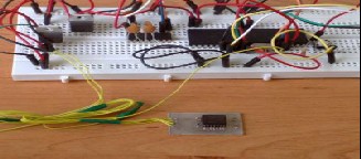
Figure 1: produced accelero meter c ircuit
Having programming of micro with respect to sensor‘s datasheet, an ‗exe‘ file is extracted to test and collect output. Measurement accuracy during the experiment is flexible so that in this trial 0.02 second is taken. Output data will be then recorded as product of gravity and the relevant ‗txt‘ file containing acceleration form will be accessible as well.

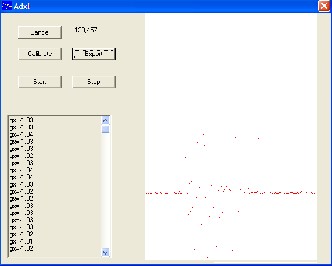
Figure 2: accele ro meter res ult dis play
It is mentionable that the sensor ADXL 202 is capable to measure acceleration in both longitudinal and lateral directions. In this work as shown in figure 3, acquired data will be accessible in longitudinal way.
of gravity. Seismic waves have low frequency but large wave length and much number of cycles.
The acceleration of an arbitrary point of earth can be
recorded by means of accelerometer based on its time adjustment, for example in intervals of 0.2 second which eventually these data would be the basis of seismic engineering. [2] [3]
In this research, an accelerometer using sensor ADXL202 and AVR (ATMEGA16) was designed and manufactured.

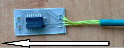
Figure 3: meas ure ment direction of accelerat ion
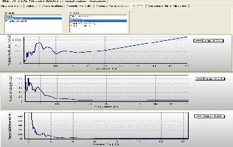
Importing text file of these points in the seismo signal software concludes to obtaining all amounts of displacement and velocity as what figure 4 depicts which is carried out through conversion of the acceleration points. Therefore the text file of displacement and velocity will become available.

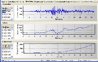
Figure 4: Graphs of acceleration, ve locity and dis placement vers us time in s eis mo s ignal
Now it would be possible to calculate these data with respect to frequency. In these graphs, the frequency range that contains values‘ peak will be used. [4] [5]

http://www. ijs er.org

Inte rnatio nal Jo urnal o f Sc ie ntific & Eng inee ring Re se arc h, Vo lume 2, Issue 12, Dece mbe r-2011 3

ISS N 2229-5518

This equation over [xi-1,xi] is cubic spline but unknown quantities of Mi still need to be determined. So they are processed through the following relations

xi  x0  ih , i  0(1)n

1 2 2 1 2 2

S (x) 

1

(xi  x)[(xi  x)
6h
 h ]M i 1 

(x  xi 1 )[(x  xi 1 )
6h
 h ]M i

 [(xi  x) f i 1  (x  xi 1 ) f i ] ,

i  1(1)n

(4)
And

M i 1

 4M i

 M i 1

 6 ( f h 2

i 1

 2 f i

 f i 1 ) ,

i  1(1)n 1

(5)
Figure 5: Graphs of acceleration, ve locity and dis placement vers us frequency in s eis mo s ignal

M 0  M n  0

M 0  M n , M1  M n 1 , f0  fn , f1  fn 1

 6  f1  f0 

2M 0  M1  h  h
 f0 

3. Mathematic va lidation

To obtain more accurate results, Spline Interpolation is used.


M  2M 

 n 1 n


6 
 fn 


fn  fn 1 


Therefore a given domain of [a ,b] is divided to sub-domains 
[xi-1,xi] where i =1(1)n; then the function is approximated by

h  h 

(6)
the polynomials with lower order in each sub-domain.[6]

(x0 , f 0 ), (x1 , f1 ),..., (xn , f n )

The interpolation in every sub-domain is linear and it is done by the variable x in (n+1) points using Lagrange linear formula. Then a spline function of order n and nodal points of x0, x1 , …, xn and correspondent function of S(x) is defined as following
S(x) is a n-order polynomial over every sub-domain [xi-1, xi],
1 ≤ i ≤ n.

S(x) and its derivatives are continuous over [a ,b]. Assuming s (xi1 )  M i1 , s (xi )  M i :

4. Programming and Simulation

A. Coding and results

Now, the results and acquired mathematical relations are
implemented by means of simulink in order to go through programming and simulating via matlab. First M-file programming and mathematical strategy for solving the problem is presented that subsequently the harmonics of a seismic wave would be determined.
In this program first of all, the data obtained from accelerometer are imported in workspace medium of matlab and then it will be executed.
spline coding is as the following :

syms x s

( x  x)3

( x  x )3

for i=1:n-1

S ( x)  i M

 i 1 M  C x  C

6hi

i 1

6hi

i 1 2

(1)

s(i)=[m(i)*((t(i+1)-

x)^3)/(6*h)]+[m(i+1)*((x-

Where C1 and C2 are integration constant and considering
interpolation conditions:

s(xi 1 )  f (xi 1 ), s(xi )  f (xi )

So that these two unknown constants can be resulted as

t(i))^3)/(6*h)]+[(y(i+1)-y(i))*(x-t(i))/h]- [h*(m(i+1)-m(i))*(x-t(i))/6]+y(i)- [m(i)*(h^2)/6];

end

for i=1:n-1 end

f  f 1

C  i i 1  (M  M )h

hi 6

i 1 i

Where s(i) is a polynomia l of order 3 which is product of

( x f  x f ) 1

C  i i 1 i 1 i  ( x M

 x M )h

interpolation between points i and i+1. Next step is coding the

hi 6

i 1

i 1 i i

(2)
main function to attain coefficients of Fourier series. [3]
Then

  2  2 

  2  2 

syms x harmA harmB

for j=1:k

A=0;

( x x)

S ( x)  ( x  x) i

h i

M  ( x  x

) ( x

xi 1 )

h i M

B=0;

i 

 6hi

1 1

 i 1



i 1

 6hi 

for i=1:n-1

A=A+(2/w)*(int(s(i)*cos(j*pi*x*2/t(n)),x,t(

 ( xi  x) f i 1 

( x  xi 1 ) f i

(3)

i),t(i+1)));

http://www. ijs er.org

Inte rnatio nal Jo urnal o f Sc ie ntific & Eng inee ring Re se arc h, Vo lume 2, Issue 12, Dece mbe r-2011 4

ISS N 2229-5518

B=B+(2/w)*(int(s(i)*sin(j*pi*x*2/t(n)),x,t(

i),t(i+1))); end harmA(j)=A; harmB(j)=B;

end

Now, due to summing the harmonics of function it would be possible to obtain expected waveform and have it compared with accelerometer data and also this waveform is served as a reference signal in simulink.
The results of M-file programming are presented as it
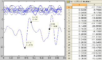
follows. First, a finite number of sequent points are analyzed as input. In the written program, k indicates harmonics number and n represents point numbers. Setting k=5 and n=10 and running the program, it can be seen that the resulted graph remarkably resembles to the main waveform. In the following figures, the left-side ones show the resulted graphs from programming and those on right-hand are concerning to the points given by accelerometer.

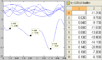
Figure 6: cons idering res ults k=5 and n=10

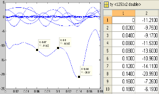
Figure 7: cons idering res ults k=10 and n=10
It can be observed that the accuracy of wave profile is being improved due to the increase in harmonics number.
Figure 8: res ults with k=10 and n=20

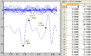
Figure 9: res ults with k=15 and n=20
The interpolation process becomes more complicated as the variations in acceleration amplitude intensify and the number of harmonics increases.

B. Simulation in simulink and its re sults

In this step, a two-branch, full-bridge inverter with four IGBT is used to obtain the predictable waveform. Similar to what was applied to the reference i.e. seismic wave, the switching method PWM is used again. [7] [8] [9]

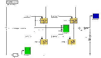
Figure 10: two-branch voltage s ource inverter in s imu lin k

http://www. ijs er.org

Inte rnatio nal Jo urnal o f Sc ie ntific & Eng inee ring Re se arc h, Vo lume 2, Issue 12, Dece mbe r-2011 5

ISS N 2229-5518

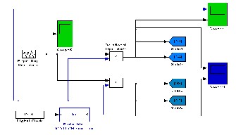
Figure 11: Control circuit of inverter for s witching of
IGBTs
The block fcn contains one input and one output to create reference signal obtained from coding results.
The basic state of input parameters and quantities for
examination and comparison are as following in which R and L represent resistance and load inductance respectively. Moreover, Fc is the carrier frequency and one or two parameters in each part are changed.
Load: R = 100 ohm , L = 0.2 H Number of points: n = 20
Number of harmonics: k = 10
Carrier Frequency: Fc = (40*k)/t(n) = 2.2 kHz
In the following figures, the top graphs show the current load of inverter and the bottom ones relate to the wave that is expected to be created by inverter.

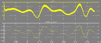
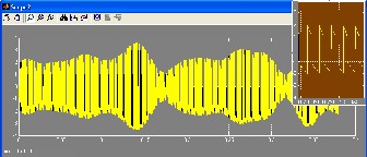
Figure 12: bas ic a mounts res ult
Figure 13: DC s ource current
The current passing through DC source has two cases in top and bottom which is similar to the reference signal so that two IGBT simultaneously i.e. either 1 and 4 or 2 and 3 get switched together to operate properly. Figure 14 shows load current supplied by reference signal which has been caused from the points having intense variation in acceleration. This time span starts at t=14 and ends up at t=14.18.

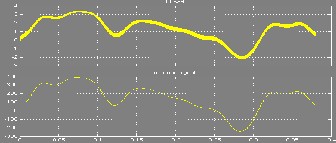
Figure 14: res ults with bas e amounts at s econd of 14 to 14.18

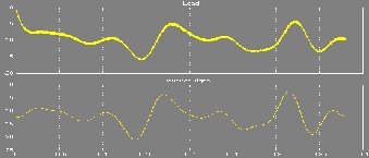
Figure 15: res ults with bas e amounts and R = 20 ohm

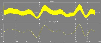
Figure 16: res ults with bas e amounts and L = 0.1 H
It is mentionable that the less proportion of inductance to resistance becomes, the more variation is caused.

http://www. ijs er.org

Inte rnatio nal Jo urnal o f Sc ie ntific & Eng inee ring Re se arc h, Vo lume 2, Issue 12, Dece mbe r-2011 6

ISS N 2229-5518

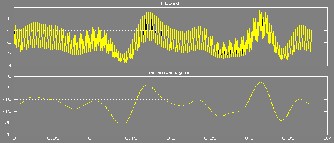
Figure 17: res ults with bas e amounts and Fc = (10* k)/t(n) =
550 Hz
It would be possible to use mosfet instead of IGBT to achieve
faster switching. [10] [11] [12] [13]

5. CONCL USION AND PROSP ECTIVE WORK

According to the presented procedure in this paper, it would be possible to create a current that it is set, for example, as supply source of a linear motor. Thereafter it can be used in practical applications such as simulation of a car shock absorber or design of earth quake table. Furthermore, considering this concept that how to create such this current, it would be feasible to utilize that for filtering unknown and unfavorable waves simultaneously in crucial or important power networks. This issue can be a topic for further researches in future.

References

[1] K. Walch, R.J. Barron J.F. Diehl, ―Design and implementation Earthquake Shake Table‖ Department of Geological and Mining Engrg and Sciences mtu.edu 2001

[2]K. Aki and M. Tsujiura, "Correlation study of near eart hquake

waves", Bull. Earthq. Res. Inst., 37, pp1959

207-231.

[3] J.B. Allen, "Short-time spectral analysis, synthesis and modifications

by discrete Fourier transform",

IEEE Trans. Acoust., Spech , Signal Processing, ASSP-25, pp 235-238

June1977.

[4] Kh. bargi, ―Principles of Earthquake Engineering‖ Tehran university

press, eighth edition 2007

[5] Kh. bargi, ―Structural Dynamics‖ Tehran University Press, fifth

edition 2008

[6] Allahvirenlu , babolian, ―Advanced Numerical Analysis‖ islamic

azad University of Science and Research press, fourth edition 2008

[7] H.J. Jiang, Y. Qin, S.S. Du, Z.Y. Yu and S. Choudhury, ―DSP Based Implementation of a Digitally-Controlled Single Phase PWM Inverter for UPS,‖ Telecommunications Energy Conference, pp. 221 – 224, INTELEC Twentieth International 4 -8 Oct. 1998

[8] J. K. Steinke, ―Use of an LC Filter to Achieve a Motor-Friendly Performance of the PWM Voltage Source Inverter,‖ IEEE Transactions on Energy Conversion, pp. 649 – 654, Volume 14, Issue 3, Sept. 1999.

[9] J. Holtz, ―pulse width modulation – A survey ‖IEEE transactions on

industrial Electronics , vol. 38,no. 5,pp. 410 -420, 1992

[10] J. Holtz, ―Pulse width modulation for electronic power conversion,‖

Proc. IEEE, vol. 82, pp. 1194–1214, Aug. 1994

[11] J. A. Houldsworth and D. A. Grant, ―The use of harmonic distortion

to increase the output voltage of a three-phase PWM inverter,‖ IEEE

Trans. Ind. Applicat., vol. 20, pp. 1224– 1228, Sept./Oct. 1984.

[12] A.M. Hava, R.J. kerkman, and T.A. Lipo, ―simple analytical a nd

graphical tools for carrier based PWM methods ― in IEEE – PESC conf.

records, st. Louis, Missouri, pp.1462 -1471, 1997

[13] M.H. Rashid ―Power Electronics Handbook‖ Academic Press 2001

http://www. ijs er.org