International Journal of Scientific & Engineering Research, Volume 4, Issue 6, June-2013 132

ISSN 2229-5518

Analysis of Simple CORDIC Algorithm Using

MATLAB

Amit Singh, Sandeep D. Bhad

Abstract — This paper presents the phenomenal work of Volder [1] who while solving the problem of navigation system evolved an algorithm named CORDIC. Since its invention, many researchers have modified and have implemented CORDIC in almost all spheres of engineering whether calculation of trigonometric functions, square root, logarithmic functions in Robotics, 3-D graphics or communication.In this paper an attempt has been made to present MATLAB implementation of simple CORDIC technique. First of all the introduction to CORDIC is presented with its basic algorithm, followed by a MATLAB code and simulation results.

Index Terms — CORDIC, DCT, DST, DHT, CZT

——————————  ——————————

1 INTRODUCTION

ith the invention of microprocessors and enhancements such as single cycle multiply-accumulate instructions and special addressing modes, and after being less cost-
ly and extremely flexible, they are not fast enough for truly demanding DSP costs .While hardware-efficient solutions are there, there has been a wide use of a class of iterative solutions for trigonometric and other transcendental functions that use only shift and addition to perform [10]. It was called Co- ordinate Rotation Digital computer (CORDIC). Since1959, when Jack Volder [1] introduced the CORDIC algorithm many papers have been published both about its applications and its analysis. The optimisation of a CORDIC processor is obtained at three interrelated levels and with a hierarchical approach, the algorithm level, the architectural level and the circuit level. Obtaining a balance between the different aspects of the prob- lem to be dealt with, available resources, speed of the circuit, accuracy, etc enables a better solution to be achieved for spe- cific applications

2 CORDIC OVERVIEW

CORDIC is an iterative algorithm for the calculation of the rotation of a two-dimensional vector, in linear, circular and hyperbolic coordinate systems, using only add and shift oper- ations. It consists of two operating modes, the rotation mode (RM) and the vectoring mode (VM). In the rotation mode a

y’= ycos θ+xsin θ (1) where (x, y) and (x’, y’) are the initial and final coordinates of the vector, respectively.
Figure 1 Rotation of a trajectory in x-y plane
The hardware realization of these equations requires four mul- tiplications, two additions/subtractions and accessing the table stored in memory for trigonometric coefficients. The CORDIC algorithm computes 2D rotation using iterative equations em- ploying shift and add operations.
Let us set n times of rotation and the rotation angle every time

is θi such that tanθi=2-i, so
vector (X, Y) is rotated by an angle θ to obtain a new vector
(X’, Y’). In every micro-rotation i, fixed angles of the value arctan(2−i ) which are stored in a ROM are subtracted or add- ed from/to the remainder angle θi , so that the remainder an-
cos 𝜃𝑖 = �
I-th rotation is expressed as (3).

1+2−2𝑖

1
(2)
gle approaches to zero (Fig. 1). In the vectoring mode, the
length R and the angle α towards the x-axis of a vector (X, Y)
are computed. For this purpose, the vector is rotated towards
the x-axis so that the y-component approaches to zero. The

𝑥𝑖+1 = 𝑥𝑖 − 𝛿𝑖 𝑦𝑖 2−𝑖 �

𝑦𝑖+1 = 𝑦𝑖 + 𝛿𝑖 𝑦𝑖 2−1 �
1 + 2−2𝑖
1
sum of all angle rotations is equal to the value of α, while the value of the x-component corresponds to the length R of the vector (X, Y). The conventional method of implementation of
2D vector rotation shown in Figure 1 using the given rotation transform is represented by the equations

x’= x cos θ − ysin θ,

1 + 2−2𝑖
𝑧𝑙+1 = 𝑧𝑖 − 𝛿𝑖 tan−1 2−𝑖 (3)
Where, after I-th rotation, the angle change is zi.The direction
of one rotation is δi, which is equal to the sign of zi, that is
δi=sign(zi).When δi=+1, rotates counterclockwise, and when
δi=-1, rotates clockwise.

International Journal of Scientific & Engineering Research, Volume 4, Issue 6, June-2013 133

ISSN 2229-5518

� 1

1+2−2𝑖

(4) is the correction factor for each level, that is, the

For i=0 to b-1 Do

rotation vector module changes of each level. For a certain
μi =sign(zi) /*μi=1 if Z > 0

length, the total correction factor is a constant. If the total se- ries of rotation is N, the total correction factor is expressed

And

<0 */

with K as (5).

𝑁−1

𝐾 = � �

𝑖=0

1
1 + 2−2𝑖
(5)
μi=-1 if Z

Zi+1=Zi- μiαm,i;

/* CORDIC Vector rotation */
Take 16-bit as an example, K = 0.607252935. We can first cor-

T T

rect the data for the operation, so that each level of operations
can be reduced to (6).
𝑥𝑖+1 = (𝑥𝑖 − 𝛿𝑖 𝑦𝑖 2−𝑖

Initialization [X Y ] =[X Y]

0 0

For i=0 to b-1 Do

X = x -m. μ y δ

𝑦𝑖+1 = 𝑦𝑖 + 𝛿𝑖 𝑦𝑖 2−1

i+1 i

i i m,i

𝑧𝑙+1 = 𝑧𝑖 − 𝛿𝑖 tan−1 2−𝑖 (6)

Yi+1 = yi+μixiδm,i

/* Scaling Operation */
From (6), it can be seen that all the operations are simplified to 1 1
add,subtract and shift operations.When given the initial input data is x0=K and y0=0, z0=θ.After n times of iteration, the re- sults are as follows:
𝑥𝑛 = cos 𝜃
𝑦𝑛 = sin 𝜃
𝑧𝑛 → 0 (7)
By the analysis of formula (7), we can see that the rotation
mode of CORDIC algorithm in circle system can be used to
calculate the input angle of the sine, cosine and so on
[6][7][8][9].

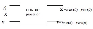
The basic block diagram of CORDIC processor is given below:
Figure 2 CORDIC Processor Block

3 MATHEMATICS OF CORDIC

The basic conventional algorithm to rotate the coordinate axis is given below:
/* CORDIC angle Conversion */

Initialization Z =θ

————————————————
• Amit Singh is currently pursuing Masters Degree programme in VLSI and Embedded System Design from Dept. of E&TC, Disha In- stitute of Management and Technology ,Raipur , Chhattisgarh, In- dia. E-mail: amit.18.singh@gmail.com.
• Sandeep D. Bhad, Asst. Professor, Deptt. of E&TC, DIMAT, Rai-
pur, India . E-mail: sandeepbhad@gmail.com

𝑋 = 𝑋, 𝑌 = Y

𝑘 𝑘

During the angle conversion phase, the angle θ is represented
as the sum of a nonincreasing sequence of elementary rotation
angles , (𝛿𝑚,𝑖 = 2−𝑖 defines a radix 2 number system, 0<=i<=b-

1)where b is the number of rotations ,which in turn depends

on the kind of precision we wanted, such that

𝑏−1

𝜃 = � 𝜇𝑖 𝛼𝑚,𝑖

𝑖 =0

In the above algorithm, the set of parameters μi(= ±1) consti-
tutes an implicit representation of θ, and b is the number of
bits in the internal register. Variable represents the rotation in
three different systems: the circular, linear and hyperbolic re- spectively .In DCT, θ is known in advance and the operation is always in Circular system only with m=1. The scaling factor
𝐾 = ∏𝛿 −1 cos tan−1 2−1 will be a constant and independent of
|μi|=1.Hence K can be computed in advance and by calculat-
ing the limit comes to be around 0.60725.All the angles in an- gle conversion contains pre computation of arc tan. So this is implemented in the form of a look-up table in hardware.

3 ALGORITHM FLOWCHART

4 RESULT

International Journal of Scientific & Engineering Research, Volume 4, Issue 6, June-2013 134

ISSN 2229-5518

Figure 3 CORDIC function with various input and output values

4 APPLICATIONS

CORDIC technique is basically applied for rotation of a vector in circular, hyperbolic or linear coordinate systems, which in turn could also be used for generation of sinusoidal wave- form, multiplication and division operations, and evaluation of angle of rotation, trigonometric functions, logarithms, ex- ponentials and Moreover, it is used in signal and image pro- cessing, digital communication, robotics and 3-D graphics. CORDIC techniques have a wide range of DSP applications including fixed/adaptive filtering and the computation of dis- crete sinusoidal transforms such as the DFT, discrete Hartley transform (DHT), discrete cosine transform (DCT), discrete sine transform (DST) and chirp -transform (CZT) .CORDIC algorithm can be used for efficient implementation of various functional modules in a digital communication system. Most applications of CORDIC in communications use the circular coordinate system in one or both CORDIC operating modes. The RM-CORDIC is mainly used to generate mixed signals, while the VM-CORDIC is mainly used to estimate phase and frequency parameters. Two of the key problems where CORDIC provides area and power-efficient solutions are: 1) direct kinematics and 2) inverse kinematics of serial robot ma- nipulators [2].

5 CONCLUSION

The result gives the CORDIC output using simple CORDIC technique. The technique can be helpful in optimization for further research and development of advanced CORDIC tech- niques. It can also be widely used in developing fast proces- sors and controllers.

REFERENCES

N´u˜nez, “A CORDIC Processor for FFT Computation and Its Im- plementation Using Gallium Arsenide Technology”, IEEE Transac- tions on Very Large Scale Integration (VLSI) Systems, Vol. 6, No. 1, March 1998, 1063–8210©1998 IEEE

[5] Lalit Bagga, Manoj Arora, R.S. Chauhan, Parshant Gupta, “Technolo- gy Roadmap of CORDIC Algorithm”, International Journal of Engi- neering, Business and Enterprise Applications (IJEBEA), IJEBEA 12-

[7] Javier Valls, Martin Kuhlmann and Keshab K. Parhi, “Evaluation of CORDIC Algorithms for FPGA Design”, Journal of VLSI Signal Pro- cessing 32, 207–222, 2002, _c 2002 Kluwer Academic Publishers. Manufactured in The Netherlands. pp. 207-222

[8] Lakshmi and A. S. Dhar, “CORDIC Architectures: A Survey”, Hindawi Publishing Corporation VLSI Design Volume 2010, Article ID 794891, 19 pages doi:10.1155/2010/794891

[9] Javier Oscar Giacomantone, “Tradeoffs in Arithmetic Architectures

For Cordic Algorithm Design”, CeTAD– Fac. De Ingeniería – UNLP [10] Ray Andraka, “A survey of CORDIC algorithms for FPGA based

0-89791-978-5/01

[1] J.E. Volder, “The CORDIC Computing Technique”, The Institute of Radio

Engineers (now IEEE), pp. 226-230 1959

[2] Pramod K. Meher, Javier Valls, Member, Tso-Bing Juang, K. Sridharan,

and Koushik Maharatna, “50 Years of CORDIC: Algorithms, Archi- tectures, and Applications”, IEEE Transactions on Circuits And Sys- tems—I: Regular Papers, Vol. 56, No. 9, September 2009, 1549-

[3] Abhishek Singh, Dhananjay S Phatak, Tom Goff, Mike Riggs, James Plusquellic and Chintan Patel, “Comparison of Branching CORDIC Implementations”, University of Maryland Baltimore County (UMBC) Baltimore, MD 21250

[4] Roberto Sarmiento, , F´elix Tobajas, Valent´ın de Armas, Roberto

Eper-Cha´ın, Jos´e F. L´opez, Juan A. Montiel-Nelson, and Antonio