International Journal of Scientific & Engineering Research, Volume 6, Issue 4, April-2015 222

ISSN 2229-5518

An Extrapolation Method for Oxygen Diffusion

Problem

Vildan Gülkaç - Department of Mathematics, Faculty of Science and Arts, Kocaeli University, Kocaeli/Turkey vgulkac@kocaeli.edu.tr

Abstract— W e consider the oxygen diffusion equation. Oxygen diffusion in a sike cell with simultaneous absorption is an important probl em. Oxygen diffusion has a wide range of medical applications. Numerical solutions of its partial differential equation are obtained by extrapolation method with the vector of values V approximating to C (diffusion) at the mesh points. And the results gave a good agreement with the previous methods [1,2,3]. And L0 stability method of analysis of the stability is also investigated.

Keywords— Oxygen Diffusion Problem, Pade approximates, finite difference, L0 stability. MSC2010 Database:65Mxx

1. Introduction

The diffusion with absorption model accounts for the presence of moving boundary which marks the furthest penetration of oxygen into the absorbing medium and also allows for an initial distribution of oxygen through the absorbing tissue. The model predictions may be used in the development of time variant radiation treatments of cancerous tumors, so that the dosage of radiation could be
injected into either from the inside or outside of the cell.
At the second level, the absorption of injected
oxygen by tissues starts. This condition causes the moving
boundary problem. The goal of this procedure is to find a balance position and to define the time dependent moving boundary position.
In one dimension, the diffusion with absorption
process is presented by parabolic partial differential
equation [1]
varied with the changing oxygen concentration. Simple

–m (1)
expressions are also presented for evaluating the surface
oxygen concentration the rate of consumption of oxygen per unit volume of absorbing tissue, and the point of
innermost oxygen penetration.
Crank and Gupta [1] studied the moving boundary
problem arising from the diffusion of oxygen into absorbing tissue. Crank and Gupta [4] also employed an uniform space grid moving with the boundary and the necessary interpolations are performed with either cube splines or polynomials, Liapis et al. [5] proposed an orthogonal collocation for solving the partial differential equation of the diffusion of oxygen in absorbing tissue. Gülkaç studied two numerical methods for oxygen diffusion problem [3]. More references to this problem can be found in references [6-16].
This paper is organized as follows in section 2 describes the oxygen diffusion problem. Section 3 describes the method and contains the extrapolation method for the
Where c(x,T) denotes the concentration of oxygen that is free to diffuse at distance x from the outer surface of medium at time T, D is a constant diffusion coefficient, and m a constant rate of consumption of oxygen per unit volume of absorbing medium. This problem has two parts.
1. Steady-state solution
When the oxygen enters through the surface
during the initial phase, the boundary conditions is given by the expression [3, 12]
(2)
where c0 is a constant.
The steady state is defined by a solution of

– (3)
which satisfies the conditions

=0, (4) where X0 the innermost extend of oxygen penetration. The required solution is obtained to be
oxygen diffusion problem. Section 4 describes stability of
(5)
extrapolation method for the oxygen diffusion problem.
Section 5 presents the numerical results and conclusions.

where
(6)

2. Desciription of Problem

Mathematical model of biological diffusion problem was made first by Crank and Gupta [1].
The procedure consists of two levels
mathematically. At the first level, the stable condition
occurs when the cell surface is isolated after the oxygen is
2. After the surface X=0 has been sealed, the position of the receding boundary is denoted by
X0(T) and problem can be expressed by the equation

– (7)

(8)

International Journal of Scientific & Engineering Research, Volume 6, Issue 4, April-2015 223

ISSN 2229-5518

(9)
.

dVN - 1 (t ) = 1 { V

- 2V

+ V } - 1

(10)
where T=0 is the time when the surface is sealed. By

dt h2

N - 2

N - 1 N

changing the variables

,
and denoting by s(t) the value of x corresponding to X0(T), the above system is (7)-(10) reduced to the following non- dimensional form [3]:
V0 and VN are known boundary values.
We can write this equation system (16) in matrix form as,

(17)

¶C = 0, x = 0, t ³ 0

¶x

C = ¶C = 0, x = s(t ), t ³ 0

¶x

and

(11)
(12) (13)

and, we can write as

dV (t ) = AV (t ) + b dt

or equation (18) can be write as

dV = AV + b dt

(18) (19)

C = 0.5(1 - x)2 , 0 £ x £ 1, t = 0

(14)
where V(t)=[V1, V2,…VN-1]T, b is a column vector of zeros
where C is concentration of the oxygen free to diffuse [1].

3. Extrapolation Method For The Oxygen Diffusion

Problem

3.1 Be converted into ordinary differential equations

and known boundary values and matrix A of order (N-1).
Equation (19) is scalar differential equation. A and b are
independent of t and V(t) satisfies the initial condition
V(0)=g, equation (19) is easily solved by method of separation of variables, to be

V (t ) = - b + (g + b )eAt

systems of partial differential equation A A

or

If the x derivative at (x, t) for is replaced by

V (t ) = - A- 1b + etA (g + A- 1b)

(20)

1 { C(x - h, t ) - 2C(x, t ) - C(x + t )} + O(h2 )

in equation (11) and x is considered a constant equation (11)
therefore, iteration equation for the equation (20) can be written follows
can be written as the ordinary differential equation,

V (t + k) = - A- 1b + e(t +k ) A (g + A- 1b)

(21)

dC(t )

= 1 { C(x - h, t ) - 2C(x, t ) + C(x + h, t )} - 1 + O(h2 )

(15)
or

V (t + k) = - A- 1b + ekA (V (t ) + A- 1b)

(22)
Subdivide the interval 0 £ x £ 1 into N equal subintervals by the grid lines xi=ih, i=0(1)N, where Nh=x and write down equation (12) at every mesh points xi=ih, i=1(1)N-1 along
Because all boundary values is zero (see eqn.(12) and eqn.(13)) then b=-1 and
time-level t. It then follows that the values Vi(t)
approximating to Ci(t) will be exact solution values of the system of (N-1) ordinary differential equations .
Therefore

V (t + k) = A- 1 + ekAV (t ) - A- 1

V (t + k) = ekAV (t ) + A- 1 (I - ekA )

(23)
(24)

dV1 (t ) = 1 { V - 2V + V } - 1

dt h2 0 1 2

The boundary values can be always be eliminated if we are concerned more, say, with stability than with a particular
numerical solution.

dV2 (t ) = 1 { V - 2V + V } - 1

(16)
Perturb the vector of initial values from g to g*. By equation

dt h2 1 2 3

.
.
(20) the solution V*(t) is

V * (t ) = - A- 1b + etA (g* + A- 1b)

(25)

International Journal of Scientific & Engineering Research, Volume 6, Issue 4, April-2015 224

ISSN 2229-5518

Let perturbation vector E(t) can be written as equation (26)
with equation (20) and (25)
Ci(t+2k) than either (32) or (33), i=1(1)N-1, V(t+2k)=(I+2kA+2k2A2)V(t)-A-1(I+2kA+2k2A2)+O(k3) (34) Comparison of equations (32), (33) and (34) shows that

V * (t ) - V (t ) = etA (g* - g)

Hence the perturbation vector
(26)
neither (32) nor (33) is accurate to terms of order k2. A
simple linear combination of (32) and (33) will however,

E(t ) = V * (t ) - V (t )

at time t is related to the initial
produce an extrapolated vector C(E) that is second order
perturbation vector E(0)=g*-g by E(t)=etAE(0). As before
E(t+k)=ekAE(t).

3.2 Extrapolation method for oxygen diffusion problem

If the exponential is approximated by its (1,0) Pade approximant, the vector of values C=[C1, C2, …, CN-1]T approximating V will be solution of the implicit backward difference equations [14]
C(t+k)=(I-kA)-1C(t)-B (27) Where A matrix defined is

and B is defined B=A-1(I-Ak)-1. Over a time-interval of 2k this gives
C(1)(t+2k)=(I-2kA)-1C(t)-A-1(I-2kA)-1 (28) Alternatively, the application of equation (27) twice, each
over a time-interval of k, leads to the implicit equations,
accurate in t, i.e. with a leading error term O(k3), namely,
C(E)(t+2k)=2C(2)(t+2k)-C(1)(t+2k)+F Where F is F=-A-1(I+2kA+2k2A2). C(E)=(I+2kA+2k2A2)C(t)+F
The algorithm for the extrapolation is therefore
(I-2kA)C(1)(t+2k)=C(t)-A-1 (35) (I-2kA)2C(2)(t+2k)=C(t)-A-1 (36) and
C(E)(t+2k)=2C(2)-C(1)+F (37)
Naturally, the extrapolated solution values are used as the starting values for the extrapolation procedure over the next two time-levels.

4. Stability of Extrapolation Method

If equation (37) is written in the form
C(E)(t+2k)=S1,0(kA)C(t)+F
=[2(I-kA)-2-(I-2kA)-1]C(t)
then
C(2)(t+2k)=(I-kA)-1C(t+k)=(I-kA)-1[(I-kA)-1C(t)-B] (29)
S1,0
(kA)=2(I-kA)-2
-(I-2kA)-1
C(2)(t+2k)=(I-kA)-2C(t)-(I-kA)-1B (30)
Therefore the symbol S

1,0

(-z) of the extrapolation method is,
C(2)(t+2k)=(I-kA)-2C(t)-A-1(I-kA)-2 (31)
2 1 1 + 2z - z2
Equations (28) and (31) are two different backwards difference schemes for calculating approximations to Ci(t+2k), i=1(1)N-1.
The binomial expansion of the matrix inverse of
(28) and (31) can be written as

S1,0 (- z) = (1 + z)2 - 1 + 2z = 1 + 4 z + 5z2 + 2z3
Division of the numerator and denominator by z2

that S1,0 (- z) ® 0 as z ® ¥ .

S1,0 (- z) < 1 for all z>0.

shows
C(1)(t+2k)=(I+2kA+4k2A2)C(t)-(I+2kA+4k2A2)A-1+O(k3) (32)
and
C2(t+2k)=(I+2kA+3k2A2)C(t)-(I+2kA+3k2A2)A-1+O(k3) (33)

Hence the extrapolation method is L0-stable. The symbol is small and negative for z > 1 + 2 , which implies that small oscillations of fluctuations could occur in the numerical
solution for

z = - kl s ¶ > 1 + 2

. In this case, visibility
But the Maclaurin expansion of exp(2kA) in
V(t+2k)=e2kAV(t)-A-1e2kA an equation giving a more accurate
reduces calculations, because S1,0(-z) is very small for these values of z. Therefore, only L0-stable methods are worth
approximation to
extrapolating.

International Journal of Scientific & Engineering Research, Volume 6, Issue 4, April-2015 225

ISSN 2229-5518

5. Numerical Results and Conclusion

In this work we proposed an efficient method of determining extrapolation by using pade approximates. We also showed the stability analysis to prove the merit of our proposed numerical scheme. As one would expect, L0-stable difference methods of third and fourth accuracy in the t can be achieved by extrapolating over considered in Crank [1].
The computation procedure showed that the present method is easy to handle with minimum error. A good agreement between the present method and previous methods was also shown.
The calculations performed with

dx = 0.05, dx = 0.1 and dt = 0.001are given in Figures 1 and

2 which shows that the values obtained are in very good

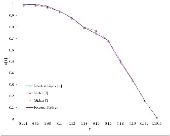
agreement with those calculated from earlier works [1, 2, 3].

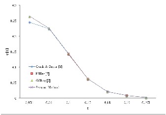
Figure 1. Position of moving boundary s(t)

Figure 2. Surface concentration c

References

[1] Crank J., Gupta RS. A moving boundary problem arising from the diffusion of oxygen in absorbing tissue. Journal of Institute of mathematical and its applications.
1972; 10: 19-33.
[2] Miller JV., Morton KW., Baines MI. A finite element moving boundary computation with an adaptive mesh. Journal of Institute of mathematical and its applications.
1978; 22:467-477.
[3] Gülkaç V. Comparative study between two numerical
methods for oxygen diffusion problem. Communications in numerical methods in engineering. 2009; 25: 855-863.
[4] Crank J., Gupta RS. A method for solving moving
boundary problems in heat flow a using cubic splines or polynomials., Journal of Institute of mathematics and its applications.1972; 10: 296-304.
[5] Liapis AI., Lipscom GG., Crosser OK. A model of
oxygen diffusion in absorbing tissue. Mathematical
modeling. 1982; 3: 83-92.
[6] Noble B. Heat balance method in melting problems, in
moving boundary problems in heat flow and diffusion. Ockendon JR., Hodkins WR.,(eds) Clarendon Press. Oxford,
1975; 208-209.
[7] Reynolds WC., Dalton TA. Use of integral methods in transient heat transfer analysis. ASME paper, 1958; 58- A;248.
[8] Hansen E., Hougaard P. On a moving boundary
problem from biomechanics. Journal of institute of
mathematical and its applications. 1974; 13: 385-398.
[9] Ahmet SG. A numerical method for oxygen diffusion
and absorption a sike cell. Applied mathematics and computation. 2006;173.
[10] Gupta RS., Kumar A. Variable time step method with
coordinate transformation. Computer methods in Applied mechanics and engineering. 1984; 44:91-103.
[11] Öziş T., Gülkaç V. Application of variable interchange method for solution of two dimensional fusion problem with convective boundary conditions.
Numerical Heat Transfer part A. 2003;44:85-95.
[12] Boureghda A. Numerical solution solution of the
oxygen diffusion in absorbing tissue with a moving boundary. Communications in Numerical Methods in Engine-ering .2006;22:933-942.
[13] Furzeland RM. A survey of the formulation and
solution of free and moving boundary problems. Brunel
University Technical report TR/76, 1977.
[14] Smith GD. Numerical solution of partial differential
equations. Clarendon press. Oxford,1985.
[15] Gupta RS., Dhirendra K. Complete numerical solution
of the oxygen diffusion problem involving a moving
boundary. Computer methods in applied mechanics and engineering.1981;29:233-239.
[16] Gupta RS. Moving grid method without interpolations. Comput. Methods Appl. Mech. Engrg.1974;4:143-152.

International Journal of Scientific & Engineering Research, Volume 6, Issue 4, April-2015 226

ISSN 2229-5518