International Journal of Scientific & Engineering Research, Volume 4, Issue 12, December-2013 1664
ISSN 2229-5518
A Survey on Spatial Association Rule Mining Technique and Algorithms for mining spatial data
Banalata Sarangi, (Prof.) Dr. Laxman Sahoo
Abstract— spatial association rule mining is an important technique of spatial data mining. Mining spatial association rule is one of the most important branches in the field of spatial data, spatial data mining can extract the spatial patterns and characteristics, general relations of spatial and non spatial data and other data features in common that hidden in spatial database. This paper describes and explains various spatial association rule mining algorithms and methods. Here we try to give a detailed survey of the existing spatial association rule mining technique based on Buffer analysis, Maximum frequent item sets based on Boolean matrix, concept lattice.
Index Terms— Data mining, Spatial mining, spatial association rule, and spatial data mining.
1 INTRODUCTION
—————————— ——————————
Data mining in general is searching for hidden and interesting patterns that may exist in generic data. Spatial data mining in particular is discovering the interesting relationships and characteristics that may exist implicitly in spatial data. Associ- ation rules analysis was only used to find out frequently ap- pearing transactions in relational database based on apriori, but with the development of geographic information technol- ogy, people have not satisfied with the traditional data mining.
2 SPATIAL ASSOCIATION RULES STUDY BASED ON BUFFER ANALYSIS
This method finds out longest groups in which object influents
each other.
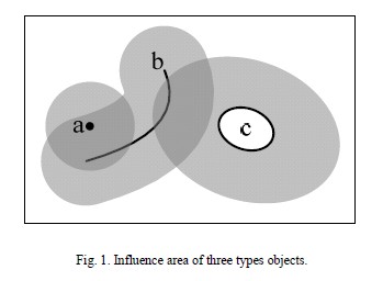
2.1 Influence area and buffer area.
All spatial objects, no matter belongs to any type, will influent surrounding objects. In this paper, the influence radius area also called buffer area. It can be said that object have some influence or contact on other objects which locate inside the influence radius area.
Theorem 1:
If a's influence radius is ra, and a's buffer area intersects with b, then it can be said that a influence on b.
Exists (b Interact (Buffer (a, ra)) = true
2.2 Support and Confidence
Formula 1:
Support(X) =
Spatial objects have bigger Support degree, means they have bigger ratio to all spatial object, and means they are more im- portant.
Formula 2:
Some spatial objects like broadcast station have very large range so frequency will not take more important to calculate support. So
• Banalata Sarangi is currently pursuing Ph.D. degree program in School of Computer engineering in KIIT University, India, E-mail: banalata1sarangi@gmail.com
Confidence-


Support(X) =
• Prof.(Dr.)Laxman Sahoo is working as Professor and Hod(Database) in School of Computer Eengineering in KIIT University, India, E-mail: laxmansa- hoo@yahoo.com
If X and Y, two type spatial objects, and their influence radius-
es are rx and rr. Function Count(X) returns the X type objects
number in spatial area, and function Count(X*(Y©ry)) returns
the X type objects number which inside Y influence area.
Formula 3
IJSER © 2013 http://www.ijser.org

Confidence(Y => X) =
International Journal of Scientific & Engineering Research, Volume 4, Issue 12, December-2013 1665
ISSN 2229-5518
Theorem-1
When the confidence of X influencing y and the confidence of y influencing X are all bigger than a threshold c%.So X and y are appearing frequently.
Min (Confidence(X => y) , Confidence(Y => X)) > c%
C% = Confidence threshold.
2.3 Basic Algorithm steps of finding Association rules:
Assume there are j kinds of spatial objects in the spatial area, AI, A2, ... , Ai' the main steps of the basic algorithm to find out the longest association groups are as following:
Step 1: Based on Formula 1 or Formula 2, pick out these types of objects which satisfy the Support Threshold s%.
Step 2: According to Formula 3, calculate Confidences of all two-tuple groups.
Step 3: Set n=2. Then, according Theorem 2 comparing the Confidence threshold c%, pick out all groups with n- ary asso- ciation. If these groups don't exist, the algorithm will exit di- rectly.
Step 4: Set n=n+ I, if n>j, then jump to step 6. Otherwise, pro-
ry, binary transaction of transaction T isexpressed as BT= (b1 b2…bm), bk∈ [0, 1], k=1…m. If ik ∈ Ti, and then bk=1, other- wise bk=0, the order of binary digits are as same as items which have been fixed. Example, Let I={1,2,3,4,5} be a set of items, if a transaction is expressed as Ti={2,3,5}, and then BTi=(01101).
DT-Digital Transaction (DT), which is the integer, the value of which would be obtained by turning binary of transaction into algorism. Example, If BT=01101, and then DT=13.
FDT- Frequent Digital Transaction (FDT), which is a digital
transaction, the support of which excess minimal Support giv-
en by users.
CDTS- Candidate Digital Transaction Section (CDTS), which is
an integral section from 3 to max, each power of 2, does not belong to CDTS.
Max=BTi1 υ BTi2…υ BTjk, each BT only expresses a kind of
item, their support excess minimal support given.
3.2 The Process of Association Rules Mining Based on
Binary
Firstly, we define some signs as follows:
IJSER
cess previous step results according to Theorem 3, pick out all
groups with n-ary association.
Step 5: If n-ary association groups don't exist, then jump to
step 6. Otherwise, store all n-ary association groups, and jump to step 4.
Step 6: Output all groups with n-ary association
2.4 Advantages of the algorithm
This algorithm reduces human intervention and suits for all shapes of spatial object.
3 SPATIAL ASSOCIATION RULE BASED ON BINARY MIN ING ALGORITHM
In areas like mobile computing there are many spatial data correlative with locations,which are very important for mobile inteligent system to extract spatial association among locations that can provide potential and useful information formobile client.this paper proposes an approach of extracting spatial association rules based on binary mining algorithm.
3.1 THE ALGORITHM OF ASSOCIATION RULES MINING BASED ON BINARY
Let I= {i1, i2…im} be a set of items, if ik I let T= {i1 ∧ i2 ∧… ∧ im} (Tk ⊆ I) be a subset of items, named a transactions. For example, let Tk= {i1, i2, i3} be a subset of items, called a trans- action. And then let D= {T1, T2…Tn}, let Tk ⊆I, (k=1…n) be a set of transactions, called Transaction Database (TD).
BT-Binary Transaction (BT), a transaction is expressed as bina-
DB: DB is used to save digital transaction.
D: data-domain of D contain “value” and “count”, “value” is
used to save digital transaction and “count” is used to save the
number of same digital transaction.
FDT: data-domain of FDT contains “value” and “count”, “val-
ue” is used to save digital transaction and “count” is used to save support of digital transaction, which excess minimal support given by users.
NFDT: data-domain of NFDT only contains “value” to save digital transaction, the support of which is under minimal support given, and then go on doing:
Step 1: Data Transformations. Transaction would be trans-
formed into digital transaction from traditional database and then digital transactions would be saved in D on descending by digital transaction.
Step 2: Creating candidate digital transaction section
(CDTS).Frequent digital transactions gained by scanning D, are used to create, which only express a kind of item.
Step 3: Forming sets of Frequent Digital Transaction (FDT).All
frequent digital transactions are searched from CDTS to save in FDT.
Step 4: Creating Digital Association Rules. Digital association
rules are created from FDT when their confidence Excess giv- en min-confidence.
3.3 The Algorithm of Association Rules Mining
Let [3, max] be a CDTS, and there are N digital transactions saved in D on descending by digital transaction, where data aren’t repeated, and the algorithm which generates digital as- sociation rules after search frequent digital transaction, is ex-
IJSER © 2013 http://www.ijser.org
International Journal of Scientific & Engineering Research, Volume 4, Issue 12, December-2013 1666
ISSN 2229-5518
pressed as follows:
(1) While (DT∈[3, max]) { (2) If (all NFDTj ⊄ DT) {
(3) While (DT_Di.value&&i_N) { (4) If (DT⊆Di.value)
(5) s_count+= Di.count;
(6) i++;}//computing support of DT
(7) If (s_count/N_support) {
(8) Delete all FDTk (FDTk⊂DT) from FDT;
(9) Write DT and s_count to FDT;
(10) }//checking frequent digital transaction
(11) Else
(12) Write DT to NFDT;} (13) DT++;
(14) }//searching all frequent digital transaction
(15) For (all DT∈FDT) {
(16) DT =FDT.value;
(17) s_count= FDT.count;
(18) Create_Rules (DT, s_count);
(19) }//generating association rules
Create_Rules (DT, s_count);
efficient than apriori, and so it made the efficiency of mobile
device be improved.
4 SPATIAL ASSOCIATION RULE BASED ON BOOLEAN MATRIX
4.1. Creating a Boolean matrix according to frequent
Length-1 item sets.
All the frequent length-1 itemsets will be generated from transaction database using the Apriori algorithm when trans- action database is scanned first time and for each frequent length-1 itemset, all the IDs of transaction records containing it need to be taken note in one array. Then the corresponding Boolean array with the length being the number of the transac- tion records in database will be created for each frequent length-1 itemset. In each array, there are only two values, ‘0’ and ‘1’. If transaction record contains frequent length-1 item- set, the value is 1 in the corresponding Boolean array, vice ver- sa.
At last, a Boolean matrix will be constructed according to all the Boolean arrays of frequent length-1 itemsets.
1) Definition 1: The corresponding Boolean array of each fre-
quent length-1 itemset Im[N] is {BT1, BT2, ... , BTn} (1�
IJSER
(1) While (sub∈[1, DT] && sub⊂DT) {
(2) For (all Di∈D) {
(3) If (sub⊆Di.value) c_count+= Di.count;
(4) i++;} //computing support of sub (5) If (s_count/c_count_confidence) (6) Display sub_DT& (~sub);
(7) sub++ ;}
3.4 Process of generating spatial association rules
The process is expressed as follows:
Step 1: Digital association rules are transformed into binary, if
digital “1” exists in some binary bits, transaction-item (ij) re- lated to each bit, and then comprehensible association rules are expressed as {i1,i2}_{i4}.
Step 2: Item (ij) of comprehensible association rules would be
renewed into spatial predicate close_to (T, Oj), and then the spatial association rules are expressed as follows:
close_to (T, O1)  close_to (T, O2) _close_to (T, O4)
Step 3: The normal spatial association rules are expressed as
follows:
n�N), where Im is the mth frequent length-1 itemset; N is the number of transaction records in database; Tn is ID of the nth Transaction record respectively; and BTn’s value is 0 or 1 only.
2) Definition 2: The Boolean matrix of frequent length-1 item-
sets IM*N is {I1 [N], I2 [N], ..., Im[N]} (1�m�M), where
Im[N] is the Boolean array with N dimensions of the mth fre-
quent length-1 itemset; M is the number of frequent length-1 item sets.
3) The pseudo codes of the first part (Fig. 1):
is_a (X, T)  close_to(X, O1)
  close_to(X, O2)
_close_to(X, O4) [30%, 80%]
Let X is an objective which is hotel, so above rule is explained as follows: When percent 80 of hotel are close to O1 (mall) and O2 (traffic-service), they are also close to O4 (bank), there are percent 30 of data accord with the rule in transaction database.
3.5 Advantages of the algorithm
The efficiency of algorithm based on binary is faster and more
Figure 2. The pseudo codes of the first part
IJSER © 2013 http://www.ijser.org
International Journal of Scientific & Engineering Research, Volume 4, Issue 12, December-2013 1667
ISSN 2229-5518
4.2 Extracting Maximum Frequent Itemsets from Boolean
Matrix
Each column in the Boolean matrix represents one transaction record. Value 0 in the column means the corresponding trans- action record contains the corresponding frequent length-1 itemset, vice versa. Therefore, the number of value 1 in each column indicates the corresponding transaction record con- tains the number of frequent length-1 itemsets together. If there is the number of transaction records with the same num- ber of value 1 being larger than the minimum support, the number of value 1 may be the size of maximum frequent item- set, vice versa. As a result, a set of values in which each one may be maximum frequent itemset’s length will be obtained. Then according to each of the values in descending order, a series of candidate itemsets will be generated from frequent length-1 itemsets and the support of each candidate itemset could be calculated according to the Boolean matrix of fre- quent length-1 itemsets. If the support of each candidate item- set is larger than the minimum support, the candidate itemset
IJSER
is frequent, vice versa. At last, if the maximum frequent item-
sets generated from the set of candidate itemsets are not emp-
ty, the size of candidate itemset is required, that is length of
maximum frequent itemset. Otherwise, it is necessary to con- tinue the previous operation to check the next value until max- imum frequent itemsets are not empty. If all the maximum frequent itemsets are empty, the maximum length of frequent itemset is one .
1) Definition 3: Max[n] is an array used for storing some values of which each may be the length of maximum frequent itemset, where n is the size of Max[n].
2) Definition 4: The set of candidate itemsets of maxi- mum frequent itemsets C is {IM1, IM2, ... , IMn}, therefore, the Corresponding Boolean matrix CMn*N is {IM1[N], IM2[N], ... , IMn[N]}, where IMn is candi- date itemset.
3) Definition 5: The support of candidate itemset C, Sup- port(C) = IM1[N] And IM2[N] And ... IMn[N]. Fig. 3 shows the example of the logical Boolean operator “And” between the Boolean arrays of candidate item sets, where “And” is the logical Boolean operator, if there exists value 0, then the calculation will be 0.
4) The pseudo codes of the second part (Fig. 3):
Figure 3. The pseudo codes of the second part
Figure 3. The logical Boolean operator of the Boolean arrays of the set of candidate itemsets
4.3 Generating All the Frequent Itemsets from Maximum
Frequent Itemsets
All the frequent itemsets could be extracted from all the max- imum frequent itemsets according to the nonempty subsets of frequent itemsets being still frequent. And the support of each frequent itemset could be calculated by Definition 5. At last, all the strong association rules can be mined from all the frequent
IJSER © 2013 http://www.ijser.org
International Journal of Scientific & Engineering Research, Volume 4, Issue 12, December-2013 1668
ISSN 2229-5518
itemsets.
4.4 Advantages of the algorithm
The run time of this algorithm was much less than the apriori. It reduces times of scanning transaction database and de- creased the number of the set of candidate itemset according to the comparision of the principles between two algorithms, so is superior to apriori.
5 SPATIAL ASSOCIATION RULE MIKNING BASED ON CONCEPT LATTICE
5.1 Definition of spatial concept lattice
Concept lattice is the core data structure in formal concept analysis. Each concept is expressed by one node in concept lattice. Formal concept is the concept which is expressed for- mally. Every formal concept includes two parts extent and intent[4].
• Extent –examples contents by concept is the set of all objects included by concept, is the set off objects included by concept.
• Intent-he description of concept is the com-
relation (generalization - specialization relation, or prose-
quence - subsequence relation ). It defines: if O1≤O2, the for- mal concept (O1,D1) is the subconcept of the formal concept (O2 ,D2 ) .It is denoted as: (O1,D1 ) ≤ (O2 ,D2 )
Each node in concept lattice is a formal concept. Their rela-
tions can be described as relation of concept.
In concept lattice, there are two different nodes C1 = (O1, D1) and C2 = (O2, D2). if C1is the sub-concept of C2 , and there is not any other node C3, which satisfies:C1 ≤C2 ≤C3,Then c1=child node of c2
Then, C1 is the child node (direct subsequence) of C2, andC2
is the father node (direct prosequence) of C1.This paper de- notes intension and extension of node C by Intension(C) and Extension(C).
5.2. GENERALIZATION OF SPATIAL RELATIONSHIP- There are two methods by which to build spatial concept lat- tice. One is to build straight from the spatial data; the other is to generalize spatial relationships into attribute relation- ships.Generalization is controlled by non-spatial data. This strategy is to generalize non-spatial data primarily and then
adjust the attribute of spatial data

mon character of all examples contented by the concept.
Formal concept analysis expresses extent and intent by the
formalized mathematical language.
Both generalization and the specialization relations
among the objects can be described by the structure of
concept lattice. Concept lattice are visualized by Hasse di-
agrams.
Process of building concept form database.
The formal context is a triple T= (O, D, R).
O is the set of objects under consideration,
D is the set of their descriptors (attributes), R is a binary relation between O and D.
There is a unique lattice structure lattice L, Galios lattice or concept lattice (Wille R 1982), corresponding to the formal concept (T (O, D, R) ). And it is generalized by a partially or- dered set.
Correspondingly, besides the set of descriptors (attributes),
Each node of lattice L is a pair (Y, X) as concept where Y is the extension and X is the intension.
Y is the set of objects of power set P (O);
X □P (D) is the set of all common attributes of objects in Y.
.Each pair (Y, X) □ P(O)×P(D) is a complete pair to relation R,
that is, it satisfies:
Y= {y□ O| x□X, x R y}
X= {x□ D| y□Y, x R y}
CS (K) denotes the set of all formal concepts of K . The fore- most structure of CS(K) is built by subconcept-superconcept
Food
Colza oil Corn
peanut Colza Rice White
Figure 4
When non spatial attributes are generalized to the higher con- cept layer, spatial information should be united, spliced and so on.The main producing area of rice and wheat united when the main producing area of corn are presented. Generalize the spatial relationship to the spatial concept layer and build the spatial concept lattice based unit.
The table below is acquired after generalizing a spatial data-
base according to Fig. 1
A: Be adjacent to a river or not
B: The yield of peanuts
C: The yield of colza’s
D: The yield of rice
IJSER © 2013 http://www.ijser.org
International Journal of Scientific & Engineering Research, Volume 4, Issue 12, December-2013 1669
ISSN 2229-5518
Suppose there’s a generalized spatial database as below
TABLE I. TABLE FOR BUILDING HASSE GRAPH
TID | A | B | C | D |
1 | A1 | B1 | C1 | D1 |
2 | A1 | B2 | C1 | D2 |
3 | A2 | B1 | C2 | D3 |
4 | A3 | B3 | C1 | D4 |
A1-Adjacent to river A2-contiguous to river A3-Far away from river B1-High yield of rice
B2-middling yield of rice
B3-low yield of rice
5.3 ASSOCIATION RULE MINING ALGORITHM BASED
ON SPATIAL CONCEPT LATTICE
Theorem 1-If node H= (X, X’) in the lattice has only one par- ent node M = (Y, Y’), then any rules foreside created from H could only be a single descriptor and for P□{X’-Y’}there exists a rule P=>X’-p without redundancy.
Theorem 2- If node H= (X, X’) in the lattice has parent nodes
with the number of d, which are M1 (Y1,Y’1),M2(Y2,Y’2),…Md(Yd,Y’d),then for any descriptor p□
{X’-(Y’1□Y’2□…□Y’d),there exist a rule P=>X’-p.The total num-
ber of rules with a single descriptor is □X’□-
□Y’1□Y’2□….□Y’d□
Theorem 3- If node H= (X, X’) in the lattice has two par-
ent nodes M = (Y1,Y’1) and M2 = (Y2,Y’2),then for Ɏ p1□{Y’1- Y’1∩Y’2&Ɏ p2□{Y’2-Y’1∩Y’2},there exist a rule p1 p2 => X’-p1 p2,and the total number of rules with two descriptor as its foreside is □Y’1-Y’1∩Y’2□ * □Y’2-Y’1∩Y’2□;
ALGORITHM
Enter- a lattice L;
Output- rule set R and rules set Rules [H] without redun-
dancy of each node H;
C1-high yieIld of coJrn SER
C2-low yield of corn
D1-High yield of of wheat
D2-Relatively high yield of of wheat
D3-middling yield of of wheat
D4-Low yield of of wheat
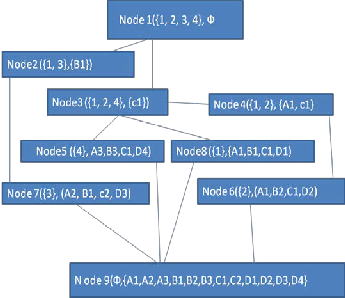
Figure-5 Hasse Diagram
FUNCTION Create Rules
For Node (H =(X, X�), k)
/ *To create rules with foreside which are descriptors with
the number of k for node H */
BEGIN
IF k=1 // If the node has only one parent node P(Y, Y�)
THEN
According to Theorem 1 that Create rules with only one
descriptor as their foreside based on Theorem 1
for ( int i=0; i<= the amount of item sets in parent nodes ;
i++ ; )
Rules[H] = Rules[H]□(yi=>X�- yi )
ENDFOR
else
if the amount of item sets in X’ <k then return else
Create rules with foreside which are descriptors with the number of k based on Theorem 2&3
for ( int j=0;j<=the amount of parent nodes of H; j++)
for ( int i=0; i<= the amount of item sets in parent nodes
:i++; )
Rules [H] = Rules [H]□(y1y2 …yi =>X�- y1y2 …yi )
ENDFOR
ENDFOR
END
PROCEDURE Create R (Lattice L, Rules R)
//Mine association rules from concept lattice
BEGIN
IJSER © 2013 http://www.ijser.org
International Journal of Scientific & Engineering Research, Volume 4, Issue 12, December-2013 1670
ISSN 2229-5518
Initialize rule set R = Ф
Go through the chain table L for storing the concept lattice, and mine association rules for each node
FOR (int i=0; i<=the amount of nodes in the chain table; i++)
R =R □Create Rules for Node (H)
ENDFOR END
5.4 Advantages of the algorithm
The algorithm can be emlimented on variety of data set having different format and is proved to be faster than apriori algo- rithm.
6. CONCLUSION
This Paper gives a detailed survey of four spatial association rule mining algorithm which uses the technique like buffer analysis, boolean matrix, binary mining, concept lattice. This paper summarise different techniques which helps the reasearcher in there work.
[12] Xu Cheng-zhi, Mei Chuan-jun,li Hao,”Spatial Association rule study based on Buffer analysis”,The *8th internatrional conference on computer science & Education,April 26-
28, 2013.Colombo, Sri Lanka.
[13] Jiawei Han, Micheline Kamber.Data mining concepts and
Techniques, Elsevier,2007.
[14] Gang FANG, Zu-Kuan WEI, Qian YIN,”Extraction of Spatial Association rules based on Binary mining Algorithm in Mo bile Computing., Proc.of the 2008 IEEE international confe rence on information and automation June 20-23, China.
[15] Koperski k, Han j. Discovery of spatial association rules in
geographic information database [A].Egenhofer M J,Herring
J R.Advances in spatial database[c], springer Verlag, berlin
1995, 47-66.
REFERENCES
IJSER
[1] R. Agrawal, T. Imielinski and A. Swami, “Mining association
rules between sets of items in large databases,” Proc. ACM
SIGMOD Int. Conf. Management Data, 1993, 207 – 216.
[2] Junming Chen, Guangfa Lin, Zhihai Yang,” Extracting Spa tial Association Rules from the Maximum Frequent Itemsets Based on Boolean Matrix”, IEEE transaction, 2011.
[3] D. Li, S. Wang, and D. Li,” Spatial Data Mining Theories and
Applications,” Beijing: Publisher of Science, 2006, pp. 32-36. [4] Jiqiang Niu, Yang Zhang, Wenjuan Feng, Lele Ren.” Spatial
Association Rules Mining for Land Use Basedon Fuzzy Con cept Lattice”, IEEE transactions,2011.
[5] J. Han and M. Kamber, “DataMining: Concepts and Tech niques,” San Mateo, CA: Morgan Kaufmann Publishers,
2000, pp.1-35.
[7] Koperski K, Han J,” Discovery of Spatial Association Rules in Geographic Information DatabAdvances in Spatial Data bases,” [C]’ LNCS951, Sp ringer-Verlag, Berlin, 1995: 47-
66. ases [A]. Egenhofer M J, Herring J R.
[8] Gang F ANG, Jiang XIONG, Cheng-Sheng TU,Ai-Ping
LUO,” An Algorithm of Mining Spatial Topology Associa tion Rules Based on Apriori”,IEEE transactions,2010,101-104.
[9] Jiangping CHEN, Fei HUANG, Rong WANG, Yi JIN,”A re search about spatial association rule mining based on concept lattice”, IEEE transactions, 2007, 5979-5982.
[10] Jiangping Chen, Pingxiang Li “An algorithm about Spatial Association rule mining based on thematic, JOURNAL OF REMOTE SENSING., May 2006,vol 23,289-293.
[11] Karthiya Banu.R, Dr. Ravanan.R, Gopal.J,”Analysis and im plementation of Association Rule Mining”,2010 IEEE Inter national conference on signal and image processing,475-
478.
IJSER © 2013 http://www.ijser.org