International Journal of Scientific & Engineering Research Volume 3, Issue 2, February‐2012 1

ISSN 2229-5518

A Study on Hubbert Peak of Australia’s Coal: A System Dynamics Approach

Sabuj Das Gupta, Md. Fakhrul Islam, Md. Rifat Rayhan, Md. Masoom Chowdhury

Abstract— American geophysicist M. King Hubbert in 1956 first introduced a logistic equation to estimate the peak and lifetime production for oil of USA. Since then, a fierce debate ensued on the so-called Hubbert Peak, including also its methodology. This paper proposes to use the VENSIM model to simulate Hubbert Peak, particularly for the Australia’s coal production. At first the peak determined with intrinsic growth rate 0.054 and ultimate re- serve 84 billion tons. The Hubbert Peak for Australia’s coal production appears to be in 2044 with a value of 778.14 million tons. Later, sensitivity analy- sis has been made with different ultimate reserves and intrinsic growth rates.

Index Terms— Hubbert peak, coal, Australia, ultimate reserve, intrinsic rate.

——————————  ——————————

1 INTRODUCTION

ccess to modern energy services not only contributes to economic growth and household incomes but also to the improved quality of life that comes with better
education and health services. All sources of energy will be needed to meet future energy demand, including coal. Coal has always been the bloodline of Australian economy. It plays a pivotal role out there. According to Australian coal association, in 2008 at $22.5 billion Australia is the largest single exporter, issued to generate 84% of Australia’s elec‐ tricity and supports 130,000 employees [1][2]. Australia is the world’s largest exporter with about 30% of world total coal export trade and 4.6% of world consumption. Besides it is Australia’s largest commodity export, earning around
$36 billion in 2009–10[3]. Australia’s success in world coal markets has been based on reliable and competitive sup‐ plies of high quality metallurgical and thermal coal. Coal is also a significant component of Australia’s domestic energy needs, accounting for around 84 per cent of Australian elec‐ tricity generation in 2008–09. As a result prediction over coal production peak value and time has become the most important issue for Australia. Hubbert peak could be used to estimate this.
In 1956, M. King Hubbert predicted that U.S. oil production
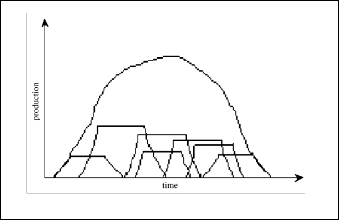
would peak in the early 1970ʹs and in 1971 Hubbertʹs pre‐ diction came true [4]. The production of oil appears to have gradual increase to a maximum output, then a long plateau and finally a slow decrease. This forms a curve which is
called Hubbert Curve. This is done by placing a small number of small fields at the beginning a large number of small fields at the end. Hubbert argued that the following logistic equation can be used to estimate oil production:
P = aQ(1− Q / R) (1)
Where P identifies the annual production of oil, ‘Q’ identi‐ fies the cumulative production which can be calculated from P, and R is the cumulative production after all reco‐ verable oil has been produced. ʺaʺ is a parameter which is called intrinsic growth rate.
This equation can be also written as
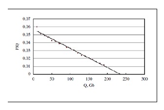
P /Q = a − aQ / R (2) Or
P /Q = a − mQ (3)
In equation (3), the parameter “mʺ shows the production of oil (a / R). Figures below show the estimation of US produc‐ tion. Only problem here is the values of ‘a’ and ‘m’ are am‐ biguous found using statistical regression for accuracy. So there is no exact value. But so far this technique is the best way to estimate the peak value of natural resources.

————————————————

 Sabuj Das Gupta is currently working as a Lecturer of EEE department in American International University-Bangladesh. His research interest includes power engineering, renewable energy, devices etc. He can be reached at the fol- lowing contacts. PH:+8801671675000. E-mail: aadi6600@gmail.com

 Md. Fakhrul Islam is currently pursuing bachelor degree program in Ameri- can International University-Bangladesh.

 Md. Rifat Rayhan is currently pursuing bachelor degree program in Ameri- can International University-Bangladesh.

 Md. Masoom Chowdhury is currently working as a Lecturer of EEE depart- ment in American International University-Bangladesh.

Fig. 1. Hubbert Curve.

IJSER © 2012 http://www.ijser.org

International Journal of Scientific & Engineering Research Volume 3, Issue 2, February‐2012 2

ISSN 2229-5518

of the target system. It has some flexibility which can be
described as:

Fig. 2. Estimation of US production.

In this paper a system dynamics approach is used to ex‐ amine the Hubbert peak of Australiaʹs coal production. In section 2, the related literature of system dynamics with the reason why it is used in order to study the Australiaʹs coal production outlook, is explained. In section 3 a system dy‐ namics model of Australiaʹs coal Hubbert peak is proposed. The model is simulated for 186 years and the results are illustrated. The value of this simple model is to help re‐ searchers in scenario building and sensitivity analysis. Here two types of sensitivity analysis have been generated. At first, the variation in Hubbert peak due to Ultimate reserve is figured out and then for different intrinsic growth rate. Thus, it offers more informative results for better energy policy decisions.

2 SYSTEM DYNAMICS

System dynamics is a field of study that Jay Forrester founded at the Massachusetts Institute of Technology (MIT) in the 1950s. The field has a long history, and has drawn from other fields as diverse as mechanical engineering, bi‐ ology, and the social sciences. In its simplest sense, system dynamics focuses on the flow of feedback (information that is transmitted and returned) that occurs throughout the parts of a system—and the system behaviors that result from those flows. For example, system dynamicists study reinforcing processes—feedback flows that generate expo‐ nential growth or collapse—and balancing processes— feedback flows that help a system maintain stability.
SD prides itself on combining human mind and the power of computers in order to overcome the barriers to learning such as dynamic complexity, limited information of prob‐ lem situation, confounding variables and ambiguity, bounded rationality, flawed cognitive maps, erroneous infe‐ rences about dynamics, and judgmental errors [5].
In this paper, SD methodology is accepted for to achieve a realistic and reflective system from a greater understanding

 The purpose is to clearly identify the problem and the factors oriented with the system.

 The relationship of all the factors with the target system is very easy to define. A sign causal dia‐ gram is drawn in order to develop the understand‐ ing of influence of the variables on each other. Ex‐ plicit concepts of SD such as flows, levels and aux‐ iliary are used in simulation model building proc‐ ess.

 After the implementation and simulation of the

model, it is possible to further analysis the sensitiv‐ ity for different scenarios that helps the policy makers more robust decision.

 However, this model is based on the historical data and cannot be 100% accurate as future may not fol‐ low the past. But clearly it gives an indication of the future production.

2.1 CAUSALITY & FEEDBACK

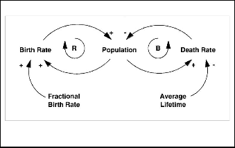
Causal loop diagrams (CLDs) are an important tool for representing the feedback structure of systems. A causal diagram consists of variables connected by arrows denoting the causal influences among the variables. The important feedback loops are also identified in the diagram. There is an Example of a Causal Loop.

Fig. 3. Causal Loop Diagram.

Variables are related by causal links, shown by arrows. In the example, the birth rate is determined by both the popu‐ lation and the fractional birth rate. Each causal link is as‐ signed a polarity, either positive (+) or negative (‐) to indi‐ cate how the dependent variable changes when the inde‐ pendent variable changes. The important loops are hig‐ hlighted by a loop identifier which shows whether the loop is a positive (Reinforcing) or negative (Balancing) feedback. The loop identifier circulates in the same direction as the loop to which it corresponds. In the example, the positive feedback relating births and population is clockwise and so

IJSER © 2012 http://www.ijser.org

International Journal of Scientific & Engineering Research Volume 3, Issue 2, February‐2012 3

ISSN 2229-5518

is its loop identifier; the negative death rate loop is counter‐
clockwise along with its identifier.
A ‘+’ link means that if the cause increases, the effect in‐ creases above what it would otherwise have been, and if the cause decreases, the effect de‐creases below what it would otherwise have been. In the example an increase in the fractional birth rate means the birth rate (in people per year) will increase above what it would have been, and a decrease in the fractional birth rate means the birth rate will fall below what it would have been. That is, if average fer‐ tility rises, the birth rate, given the population, will rise; if fertility falls, the number of births will fall.
A ‘-’ link means that if the cause increases, the effect de‐ creases below what it would otherwise have been, and if the cause decreases, the effect increases above what it would otherwise have been. In the example, an increase in the aver‐age lifetime of the population means the death rate (in people per year) will fall below what it would have been, and a decrease in the average lifetime means the death rate will rise above what it would have been. That is, if life expectancy increases, the number of deaths will fall; and if life expectancy falls, the death rate will rise.

2.3 LEVEL AND RATE

Although CLD causes in improved communication and comprehensiveness among users, only a map of causal in‐ fluences and feedback loops is not enough to determine the dynamic behavior of a system. There are two variables re‐ quired for simulating all elements inside a system, level and rate. The ʹlevelʹ refers to a given element within a spe‐ cific time interval, e.g. inventory level on December 2011 or current total students in a university and so on. Meanwhile, the rate reflects the extent of behavior of a system, such as hourly production volume, and daily sales turnover. In simple words ‘level’ means‐ an accumulation or intrigration of information & ‘rate’ means‐ an increasing or decrecreas‐ ing amount of flow. A time factor is the main concern. Specifically, the differences between the level and the rate depend on whether the element contains a time factor or not [6]. The level is calculated from the difference between a rate variable that increases the level and a rate variable that reduces the level. A value of level (an accumulated rate) can be identified easily, but a rate is not easy to be identified. The level and the rate can be formulated using the stock‐flow diagram (SFD) for a simulation test.

3 SYSTEM DYNAMICS MODEL OF HUBBERT PEAK

FOR AUSTRALIA’S COAL

A simple SD model is implemented based on Mr. Hubbert’s equation. Figure 4 shows the casual loop diagram of Hub‐
bertʹs equation. The explanation of this loop is that an in‐

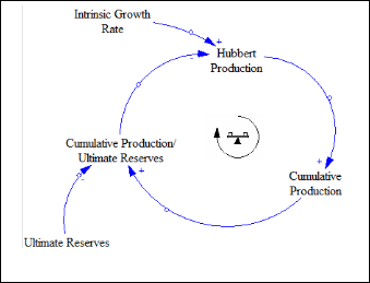
crease in Hubbert Production causes a rise in cumulative production. This increase with regard to the amount of ul‐ timate reserves, cause an increase in “cumulative produc‐ tion/ultimate reserves” ratio. As this ratio rises in the pres‐ ence of the intrinsic growth rate, the production decreases due to resource depletion.

Fig. 4. Causal loop Diagram of Hubbert Peak.

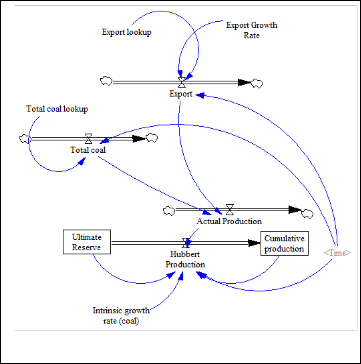
A time horizon of 186 years is defined to show the history of Australia’s coal production and its changes in the future. Two levels have been developed in this model, (1) Ultimate Reserve and (2) Cumulative Production. The Ultimate Re‐ serve does not have any inflows. This is because coal is created in geologic time. Thus, for all practical purposes, the total amount of oil is assumed to be constant. The Ulti‐ mate Reserves are conducted into the Cumulative Produc‐ tion with the rate of Hubbert production which is affected by the intrinsic growth rate. Based on Australia’s coal data, the intrinsic growth rate is 0.054. The historical data for Export and total coal (Black Coal & Brown Coal) are added with lookup variable which are named Export lookup and Total coal lookup respectively. The data is obtained from Australian commodity statistics 2009 & 2010 which is pub‐ lished by ABARES [7]. The modelʹs equations are given in the Appendix.
The model shows that Australia coal production will reach its peak in 2044 with 778.141million tones/year as shown in figure 6. This model is free from all type of policies. In the Australian energy projections to 2029‐30 the primary ener‐ gy consumption by fuel the use of coal is reduced by an‐ nually 0.8% and 0.7% for black coal and brown coal respec‐ tively [8]. There will be a right shift in the Hubbert peak curve if this policy is considered. The total economic reco‐ verable black and brown coal reserve for Australia is 84.217 billion tons [9]. Here this paper considers recoverable black coal and brown coal resources in Australia as 84 billion

IJSER © 2012 http://www.ijser.org

International Journal of Scientific & Engineering Research Volume 3, Issue 2, February‐2012 4

ISSN 2229-5518

tons. The value of export growth rate is used as 2.4% per year taken from the ABARES. One more assumption is con‐ sidered regarding the total coal. At presently, because of the CO2 emissions the use of coal is discouraged in Australia. Hence, no growth rate is used for the total coal amount which means no further increase of domestic consumption.

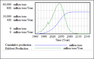
Fig: 5. Stock-flow Diagram of Hubbert Peak.

TABLE 1

SIMULATION RESULTS OF HUBBERT PRODUCTION RATE AND CUMULATIVE PRODUCTION

3.1 SENSITIVITY ANALYSIS

The behavior of the model is important and informative under some scenarios as implemented in this paper. Ulti‐ mate Reserve and the Intrinsic Rate are the very difficult to figure out for a range of time. There is a big disparity in these values from source to source. Hence, in the analysis of coal production, first scenario is about Ultimate Reserves (UR). Three different amounts are used for UR 74000, 84000 and 94000 million tons. Figure 7 and Table 2 show the be‐ havior of Australia’s coal production under these condi‐ tions. The results show that when the ultimate reserves vary from lower to higher amount, with the same intrinsic growth rate, the production peak will occur in longer time with higher production amount. In the Figure 7 the blue, green and black lines are indicating UR 74000, 84000 and

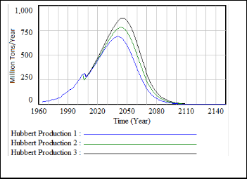
94000 million tons respectively.

Fig. 6. The Stock-flow Diagram of Hubbert Peak.

Fig. 7. Hubbert Production at Different UR.

IJSER © 2012 http://www.ijser.org

International Journal of Scientific & Engineering Research Volume 3, Issue 2, February‐2012 5

ISSN 2229-5518

TABLE 2

ILLUSTRATION OF HUBBERT PEAK UNDER DIFFER- ENT ULTIMATE RESERVES.

The Hubbertʹs equation is highly dependent on the intrinsic growth rate. Here, this parameter is changed to perform a sensitivity analysis. Figure 8 and Table 3 show the results of this sensitivity analysis. Three different models have been implemented with different intrinsic growth rate. The three values are 0.054, 0.064 and 0.074. The results show that when the intrinsic growth rate varies from lower to higher amount, with the same ultimate reserves, the production peak will occur in lower time with higher production amount. In the Figure 8 the blue, green and black lines are indicating intrinsic growth rate 0.054, 0.064 and 0.074 re‐ spectively.

Fig 8: Hubbert Production at Different Intrinsic Growth Rates.

TABLE 3

ILLUSTRATION OF HUBBERT PEAK UNDER DIFFER- ENT INTRINSIC GROWTH RATES.

4 EPILOGUE

Australia is the fourth largest producer, the largest expor‐ ter, and has the fourth largest reserves of coal in the world. Coal accounts for around three quarters of Australia’s elec‐ tricity generation, with coal‐fired power stations located in every mainland state. In export markets, coal remains the fastest growing fuel, driven by strong investment in coal‐ fired power stations in China and other developing econo‐ mies. Considering these issues the question is when the Hubbert peak would happen about Australia’s coal. In this study it is shown that the time is in the year 2044. Australi‐ an and international energy policy makers must be aware of this shortage of natural resources of Australia after ap‐ proximately 2044. Further, within Australia, the share of coal in the energy mix is expected to decrease with the Re‐ newable Energy target and a proposed emissions reduction target. Government and industry initiatives are expected to play important roles in accelerating the construction, dem‐ onstration and commercial deployment of large‐scale inte‐ grated carbon capture and storage projects. This SD model gives the opportunity to include these policy changes and hence the sensitivity analysis, which helps the policy mak‐ ers to make robust decisions.

REFERENCES

[1] International Journal of Coal Geology 85 (2011) 23–33 www.elsevi e r.com/locate/ijcoalgeo

[2] Australian coal association; Coal Facts Australia 2008, http://www.australiancoal.com.au/resources.ashx/Publica tions/7/Publication/6C91AB6A13D9D31F5D15F5A816354C7A/CO AL_FACTS_AUSTRALIA_2008_Feb08‐4.pdf

[3] Minister for resources & energy: http://minister.ret.gov.au/MediaCentre/Speeches/Pages/ CommitteefortheEconomicDevelopmentofAustralia.aspx

[4] Hubbert, M.K., 1956. Nuclear energy and the fossil fuels.

Drilling and Production Practice, 1st Ed.The American

Petroleum Institute, New York, pp: 7 – 25

[5] Sterman, J. D. 2000. Busyness Dynamics: systems thinking and modeling for a complex world. Irwin/McGraw‐Hill, ISBN 0‐07‐231135‐5

[6] Examining the Hubbert Peal of Iran’s Crude Oil: A

System Dynamics Approach. European Journal of

Scientific Research ISSN 1450 –216X Vol.25

No.3(2009), pp. 437‐447

[7] Australian Bureau of Agricultural and Resource Economics and Sciences (ABARES)2010. Australian Commodity Statistics 2010. Table 244. Available at http://adl.brs.gov.au/data/warehouse/pe_abares99001762

/ACS_2010_part2.pdf

[8] Australian energy projections to 2029‐2030, Available at

http://adl.brs.gov.au/data/warehouse/pe_abarebrs99014434/energ y_proj.pdf

[9] U.S. Energy Information Administration (2005).

ʺInternational Energy Statistics.ʺ Retrieved 8 May 2010, http://tonto.eia.doe.gov/cfapps/ipdbproject/

IEDIndex3.cfm?tid=1&pid=7&aid=6

IJSER © 2012 http://www.ijser.org

International Journal of Scientific & Engineering Research Volume 3, Issue 2, February‐2012 6

ISSN 2229-5518

APPENDICES

IJSER © 2012 http://www.ijser.org