International Journal of Scientific & Engineering Research, Volume 3, Issue 1, January-2012 1
ISSN 2229-5518

A Simplified Pipeline Calculations Program: Isothermal Gas Flow (2)

Tonye K. Jack

Abstract — and Program Objective -The familiarity and user friendliness of the Microsoft Excel TM spreadsheet environment allows the practicing engi- neer to develop engineering desktop companion tools to carry out routine calculations. A Multitask single screen gas pipeline sizing calculation program is developed in Microsoft Excel TM. Required equations, and data sources for such development is provided.

Index Terms— Isothermal pipeline design, pipe sizing, piping program, gas pipelines, engineering on spreadsheet, spreadsheet solutions.

1 INTRODUCTION

——————————  ——————————

Gas pipelines are employed for meeting various energy needs. Calculations for the design of such gas piping can often involve repetitive calculations whether for simple horizontal straight pipelines or pipelines for complex terrains. Advances in computer applications for piping design have created several off-the-shelf can programs, for which cost might be a limitation to their uses for certain, quick-check calculations. Microsoft Ex-

Flow rate:

Where,

G = γAV (6)

(5)

cel TM with its Visual Basic for Applications (VBA) automation tool can be used to develop a multi - functional single screen desktop tool to carry out such calculations.

γ = P/RT = ρg (6a)

The General Relation for evaluating such gas lines is given by equation (7).

2 REQUIRED GENERAL EQUATIONS FOR ISOTHERMAL

G 2 RT  fL 

 P1 

FLOW

P1  P 

2 2   

Ln 

(7)

Pipe cross-sections are of Circular types for which the applica- ble relations are:

2 g A

 D 

 P2 

Reynolds Number:

Re 

VD



(1)

3 FLUID PROPERTIES FUNCTIONS

A database of physical properties of typical piped gases can be developed using Microsoft Excel TM Functions category. The

Velocity: Area:

Friction factor:

V 

D2

A 

(2) (3)

developed functions are then available as drop down lists in

the Functions option of the Toolbar INSERT menu. Yaws, [2],

[3], [4] provides density, and viscosity data as functions of temperature.

As an example, the [5], derived curve-fitted gas viscosity rela- tionship for Methane (CH4), as a function of temperature is:

For Laminar Flow,

f  64

(4)

  A  BT  CT 2

(9)

For Turbulent Flow, f, is obtained by the Colebrook-White equation. Method of solution described in [1], uses the goal seek option in Microsoft ExcelTM.

Where, A= 15.96, B= 0.3439, C=-8.14 E-05

The unit of viscosity is in micro-poise, which can be converted

to Ns/m2 by multiplying by 1E-6:

Thus, the revised equation is:

 

1  2Log  D 

2.51 



g  10

A  BT  CT 2 

(9a)

f 2  3.7

 e 

The temperature, T, in ―(9),‖ is in Kelvin (K). The program can be developed to handle temperature data in Centigrade (oC) with a built-in conversion option.

http://www.ijser.org
International Journal of Scientific & Engineering Research, Volume 3, Issue 1, January-2012 2
ISSN 2229-5518

The ALIGNAgraphics [6], structured naming convention for the fluid properties functions described in [1], is applied, i.e.

Name of property_ (temperature)

For Methane: rhoMethane (temperature)

viscoMethane (temperature)

Where rhoMethane, and viscoMethane are the function

APPENDIX

Appendix A – Solution Method

From the General Relation – ―(7),‖: i.e.

names for Methane gas density and gas viscosity respectively.

P2  P2

 G RT  fL  2

 P1 

The program developer could also adopt the chemical formula 1

2 g 2 A2

 D  

Ln 

of the fluid type, particularly in cases of long fluid property

names as in some hydrocarbons. Thus, using Methane as ex-

ample, the following gas density function name will apply:

rhoCH4(temperature).

Let

 

G 2 RT Z 

 2 

g 2 A2

(10)

4 APPLICATION EXAMPLE

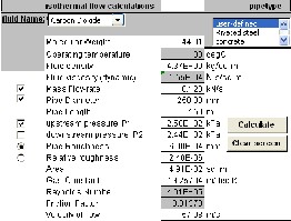
Carbon Dioxide flows isothermally at 30oC through a horizontal

250 mm diameter pipe at the rate of 0.12kN/s. If the pressure at a

Then,

 ZfL 

P2  P2 

 P1 

section 1 is 250 kPa, find the pressure at a section 2, which is 150 m 1

2  D

  2ZLn 

downstream? Take that: Pipe Roughness = 6 x 10-4 m.

 

 2 

(11)

 P 

 ZfL  

P2  2ZLn 1   

  P2 

(12)

 P2 

 D  

From ―(12),‖ neglecting the second term on the Left-Hand

Side, i.e.

 P 

ZLn 

 P2 

yields

P  P2

  ZfL  2

Nomenclature

2  1



 

 D 

(13)

P1 Upstream pressure (kPa).

P2 Downstream pressure (kPa ).

G Mass Flowrate (KN/s).

g Gravity constant (m/s2).

A Area (m2).

Then use this value of P2 to replace the P2 term in the neg- lected item, and solve for P2 on the lef-hand side of ―(11),‖.

Repeat for P1 to obtain:

f Friction factor

P   ZfL   P2  2

(14)

D Pipe internal diameter (m)

L Pipe section length (m).

M Molecular Weight

γ Specific weight (kN/m3).

ρ Gas density (kN-s2/m4).

V Velocity of flow (m/s).

R Gas constant (m/degK ).

T Temperature, (oC) or (K)

1   2 

 D  

Appendix B – A Clip of Excel VBA subroutines for stringing cell values

Option Explicit
Dim M As Double, D As Single, d1 As Single, Vel As Single, visco As Sin-

http://www.ijser.org
International Journal of Scientific & Engineering Research, Volume 3, Issue 1, January-2012 3
ISSN 2229-5518
gle
Dim L As Variant, Rho As Single, f As Single, A As Single, T As Single
Dim Mw As Single
Sub isothermalpipeType()
If Sheets("isothermal compressibleFlow").Range("K12") = 1 Then
Sheets("isothermal compressibleFlow").Range("D13") = ""
ElseIf 2 <= Sheets("isothermal compressibleFlow").Range("K12") And
Sheets("isothermal compressibleFlow").Range("K12") <= 10 Then
Sheets("isothermal compressibleFlow").Range("D13") = Sheets("isothermal compressibleFlow").Range("Q19")
End If
End Sub
Sub isothermalMolecularWeight()
If Sheets("isothermal compressibleFlow").Range("K7") = 1 Then
Sheets("isothermal compressibleFlow").Range("D4") = ""
ElseIf 2 <= Sheets("isothermal compressibleFlow").Range("K7") And
Sheets("isothermal compressibleFlow").Range("K7") <= 52 Then
Sheets("isothermal compressibleFlow").Range("D4") = Sheets("isothermal compressibleFlow").Range("Q17")
End If
End Sub
'Perform isothermal compressible flow pipe sizing calculations
'Circular pipeline section calculations
Sub Isothermalcircular()
'given M, P1, D, L, viscosity, relative roughness, upstream pressure P2 unknown
If Sheets("isothermal compressibleFlow").Range("K8").Value = True And Sheets("isothermal compressibleFlow").Range("K9").Value = True And Sheets("isothermal compressibleFlow").Range("K10").Value = True And Sheets("isothermal compressibleFlow").Range("K14").Value = 1 Then
Sheets("isothermal compressibleFlow").Range("D6") =
Sheets("isothermal compressibleFlow").Range("R18")
Sheets("isothermal compressibleFlow").Range("D13") = Sheets("isothermal compressibleFlow").Range("R19")
Sheets("isothermal compressibleFlow").Range("D15") = Sheets("isothermal compressibleFlow").Range("R24")
Sheets("isothermal compressibleFlow").Range("D16") =
Sheets("isothermal compressibleFlow").Range("R29")
Sheets("isothermal compressibleFlow").Range("D19") = Sheets("isothermal compressibleFlow").Range("R25")
Sheets("isothermal compressibleFlow").Range("D17") = Sheets("isothermal compressibleFlow").Range("R30")
Sheets("isothermal compressibleFlow").Range("R11").GoalSeek Goal:=0,
ChangingCell:=Sheets("isothermal compressibleFlow").Range("R7") Sheets("isothermal compressibleFlow").Range("D18") =
Sheets("isothermal compressibleFlow").Range("R31")
Sheets("isothermal compressibleFlow").Range("D12") = Sheets("isothermal compressibleFlow").Range("R28")
Sheets("isothermal compressibleFlow").Range("D4") =
Sheets("isothermal compressibleFlow").Range("Q17")
'given M, P1, D, L, viscosity, absolute roughness, upstream pressure P2 unknown
ElseIf Sheets("isothermal compressibleFlow").Range("K8").Value = True
And Sheets("isothermal compressibleFlow").Range("K9").Value = True And Sheets("isothermal compressibleFlow").Range("K10").Value = True And Sheets("isothermal compressibleFlow").Range("K14").Value = 2 Then
Sheets("isothermal compressibleFlow").Range("D6") =
Sheets("isothermal compressibleFlow").Range("S18")
Sheets("isothermal compressibleFlow").Range("D14") = Sheets("isothermal compressibleFlow").Range("S20")
Sheets("isothermal compressibleFlow").Range("D15") = Sheets("isothermal compressibleFlow").Range("S24")
Sheets("isothermal compressibleFlow").Range("D16") = Sheets("isothermal compressibleFlow").Range("S29")
Sheets("isothermal compressibleFlow").Range("D19") = Sheets("isothermal compressibleFlow").Range("S25")
Sheets("isothermal compressibleFlow").Range("D17") = Sheets("isothermal compressibleFlow").Range("S30")
Sheets("isothermal compressibleFlow").Range("S11").GoalSeek Goal:=0, ChangingCell:=Sheets("isothermal compressibleFlow").Range("S7")
Sheets("isothermal compressibleFlow").Range("D18") = Sheets("isothermal compressibleFlow").Range("S31")
Sheets("isothermal compressibleFlow").Range("D12") = Sheets("isothermal compressibleFlow").Range("S28")
Sheets("isothermal compressibleFlow").Range("D4") = Sheets("isothermal compressibleFlow").Range("Q17")
End If
End Sub

REFERENCES

[1] T.K. Jack, ―A Simplified Pipeline Calculations Program: Liquid Flow (1)‖, International Journal of Scientific & Engineering Research, submitted for publi- cation. (Pending publication).
[2] C.L. Yaws, ―Correlation constants for Chemical Compounds‖, Chemical Engi- neering, pp. 79-87, Aug. 16, 1976
[3] C.L. Yaws, ―Correlation constants for Liquids‖, Chemical Engineering, pp.127-
135, Oct.25, 1976
[4] C.L. Yaws, ―Correlation constants for Chemical Compounds‖, Chemical Engi- neering, pp.153-162, Nov. 22, 1976
[5] C.L. Yaws, Physical Properties, McGraw Hill, 1977
[6] AlignaGraphics Co., Pipeline Sizing Program, Pipedi User Manual, 1998
[7] J.B. Evett, 2500 Solved Problems in Fluid Mechanics and Hydraulics, McGraw-Hill,
1989
[8] A. Esposito, Fluid Power with Applications, Prentice Hall, 1980 [9] R.N. Fox, Introduction to Fluid Mechanics, Wiley, 1992.
[10] R.W. Miller, Flow Measurement Engineering Handbook, McGraw-Hill, 1985
[11] R.H. Perry, and D.W. Green, (eds), Perry’s Chemical Engineers’ Handbook, 6th edn., McGraw-Hill, 1984
[12] V.L. Streeter, Fluid Mechanics, McGraw-Hill, 1983

Biographical notes

T. K. Jack is a Registered Engineer, and ASME member. He worked on rotating equipment in the Chemical Fertilizer industry, and on gas tur- bines in the oil and gas industry. He has Bachelors degree in Mechanical Engineering from the University of Nigeria, and Masters Degrees in Engi- neering Management from the University of Port Harcourt, and in Rotat- ing Machines Design from the Cranfield University in England. He was the Managing Engineer of a UK Engineering Software Company, ALIG-

Nagraphics and the developer of a Pipeline sizing program, ―PipeDi‖. He

http://www.ijser.org

International Journal of Scientific & Engineering Research, Volume 3, Issue 1, January-2012 4

ISSN 2229-5518

is a consultant to the Seltrolene Co. and a University Teacher in Port Har court, Rivers State, Nigeria, teaching undergraduate classes in Mechanical Engineering. He can be reached by Email:- tonyekjack@yahoo.com

http //www 11ser org