International Journal of Scientific & Engineering Research,Volume 3, Issue 6, June-2012 1
ISSN 2229-5518
A Nonlinear Fuzzy PID Controller via Algebraic Product AND - Bounded Sum OR - Algebraic Product Inference
B. M. Mohan, NeethuKuruvilla
Abstract—This paper reveals a mathematical model of the simplest fuzzy PID controller which employs two fuzzy sets (negative and positive) on each of the three input variables (displacement, velocity and acceleration) and four fuzzy sets ( -2, -1, +1, +2) on the output variable (incremental control). L-type, Γ-type and ![]() -type membership functions are considered in fuzzification process of input and output variables. Controller modeling is done via algebraic product AND operator-bounded sum OR operator-algebraic product inference method- Center of Sums defuzzificatiion process combination. The model obtained in this manner, turns out to be nonlinear, is analyse d finally.
-type membership functions are considered in fuzzification process of input and output variables. Controller modeling is done via algebraic product AND operator-bounded sum OR operator-algebraic product inference method- Center of Sums defuzzificatiion process combination. The model obtained in this manner, turns out to be nonlinear, is analyse d finally.
Index Terms—PID control, nonlinear control, fuzzy control, mathematical modeling, algebraic product, bounded sum, center of sums
(CoS).
————————————————————
ONVENTIONAL (linear) PID controllers have been in extensive usage in industrial automation and process control. The reason behind this is their ease of design, low
cost, simplicity of operation, inexpensive maintenance and
effectiveness for most linear systems. These controllers generally do not work well for nonlinear systems, higher order linear systems and systems which are complex and vague having no precise mathematical models. To overcome this difficulty, various types of modified linear PID controllers such as auto tuned and adaptive PID controllers have been developed. Alternatively, controllers employing fuzzy logic have also been implemented sometimes.
Let us now take a look at the historical developments in fuzzy control technology. A fuzzy PID controller has been constructed (Wang and Kwok, 1992) by combining a fuzzy PD controller and a fuzzy I controller in parallel. It has been shown (Mizumoto, 1995) that PID controllers can be realized by product-sum-gravity method and simplified fuzzy reasoning method. A new fuzzy PID controller structure has been proposed (Qiao and Mizumoto, 1996) and a parameter adaptive method via peak observer has been presented to tune the
parameters of the fuzzy controller on-line. Analyrical structure for a fuzzy PID controller and its BIBO stability analysis has been studied (Misir et al, 1996). Fuzzy PI and fuzzy PD controllers have been combined in cascade to get a fuzzy PID controller (Kim and Oh, 2000).
In order to improve the performance in transient and steady![]()
![]() B. M. Mohan is currently working as a Professor in the Department of Electrical Engineering in Indian Institute of Technology Kharagpur, India. E-mail:mohan@ee.iitkgp.ernet.in
B. M. Mohan is currently working as a Professor in the Department of Electrical Engineering in Indian Institute of Technology Kharagpur, India. E-mail:mohan@ee.iitkgp.ernet.in![]() NeethuKuruvillais currently pursuing her MastersDegree Program in Control SystemsEngineering in the Dept of Electrical Engg, Indian Institute of Technology Khargapur,India. E-mail: kuruvilla.neethu89@gmail.com
NeethuKuruvillais currently pursuing her MastersDegree Program in Control SystemsEngineering in the Dept of Electrical Engg, Indian Institute of Technology Khargapur,India. E-mail: kuruvilla.neethu89@gmail.com
states, an adaptive method via function tuner has been developed (Woo et al, 2000) to tune the scaling factors of the fuzzy controller online. A tuning method, based on gain margin and phase margin specifications, has been proposed (Xu et al, 2000) for determining the parameters of the fuzzy PID controller. Several forms of decomposed PID fuzzy logic controllers have been tested and compared (Golob, 2001). A function based evaluation has been proposed (Hu et al, 2001) for a systematic study of fuzzy PID controllers. An adaptive method via relative rate observer has been proposed (Guzelkaya et al, 2003) for tuning the scaling factors of the fuzzy logic controller in an on-line manner.
Mohan and Sinha (2006) have shown that algebraic product triangular norm - bounded sum triangular co-norm - algebraic product inference method –CoSdefuzzification method combination leads to a linear fuzzy PID controller. Mohan and Sinha (2008a) have shown that the analytical structures of fuzzy PID controllers derived via minimum triangular norm are not suitable for control. Mohan and Sinha (2008b) have introduced an analytical structure for fuzzy PID controller by employing algebraic product triangular norm, bounded sum triangular co-norm, minimum inference method and CoSdefuzzification method. They also have derived conditions for BIBO stability using Small Gain theorem. Since linear controllers are no better than nonlinear controllers in controlling nonlinear and complex plants, in this paper an attempt is made to derive anonlinear fuzzy PID controller using the same combination (i.e., algebraic product AND- bounded sum OR-algebraic product inference- CoSdefuzzification) and modified output membership functions.
The paper is organized as follows: The next section deals
with fundamental components of a typical fuzzy PID controller. Section 3 presents a mathematical model of nonlinear fuzzy PID controller. Properties of the model are
IJSER © 2012
International Journal of Scientific & Engineering Research,Volume 3, Issue 6, June-2012 2
ISSN 2229-5518
discussed in Section 4. Section 5 concludes the paper.
![]()
The incremental control signal generated by a discrete time PID controller is given by:
given by:
v(k) ={d(k)- d[(k-1)]}/T(2)
d(k) = e(k) (3)
a(k) = {v(k)- v[(k-1 )]}/T (4)
e(k) is the error signal, r(k) is the reference command, y(k) is
u(k )
u(k )
u(k 1)
the plant output, k is the sampling instant, and T is the![]()
K d v(k )
K d d (k )
K d a(k ) (1)
sampling period. Eq.(1) is known as 'velocity algorithm' and is
P I D
where K d , K d and K d are respectively the proportional,
P I D
widely used. The principal structure of a fuzzy PID control, see Fig.1, consists of the following components:
integral and derivative constants of a digital PID controller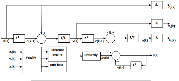
and velocity v(k), displacement d(k) and acceleration a(k) are
Fig. 1. A typical fuzzy PID controller
Let ds(k), vs(k) and as(k) be thescaled versions of d(k), v(k) and
a(k) respectively. Then
ds(k)=Sdd(k) (5)
vs(k)=Svv(k) (6)
0
(d l )
Ld ds ld
as(k)=Sa a(k) (7)
s d l d l

(9)
whereSd, Sv and Sa are the scaling factors which play a role
D 2l d s d
similar to that of
K d , K d and K d in a conventional PID
1 ld
ds Ld
P I D
controller.
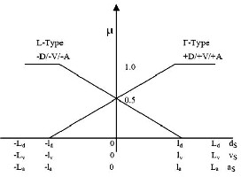
Fuzzification process converts crisp values of controller scaled inputs into fuzzy sets that can be used by the inference engine (refer Section 2.4) to activate and apply the control rule.
As shown in Fig.1, fuzzy PID controller has three
scaledinputs: ds(k), vs(k) and as(k). These inputs are fuzzified by
L-type and Γ-type membership functions as illustrated in Fig.
2. These membership functions on ds(k) are defined by:
0 Ld ds ld
( d s
D 2l
ld )
ld ds ld
(8)
Fig. 2. Input membership functions
1 ld
ds Ld
IJSER © 2012
International Journal of Scientific & Engineering Research,Volume 3, Issue 6, June-2012 3
ISSN 2229-5518
It may be noted that
(10)
![]()
![]()
![]()
D D 1
![]()
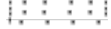
Membership functions on vs(k) and as(k) can be defined in a similar manner. The membership functions (L-type, ![]() and Γ-type) on Δu(k) are shown in Fig. 3. The constants ld,
and Γ-type) on Δu(k) are shown in Fig. 3. The constants ld,
lv, la, Ld, Lv, La, lu,, Lu and w are to be chosen by the designer.
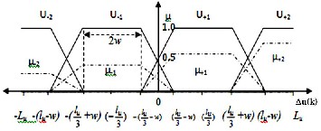
Fig. 3. Output trapezoidal membership functions (reference fuzzy sets: U-2, U-1, U+1, U+2; inferred fuzzy sets: u-2, u -1, u+1, u+2 obtained via algebraic product inference)
The following control rules are considered in terms of the aforementioned input and output fuzzy sets:![]()
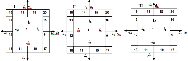
Fig.4. Regions of input
Notice that the control rules are nonlinear as the output fuzzy
sets are not linearly related to the input fuzzy sets.
Overall value of incremental control output variable is computed by the inference engine by considering the individual contribution of each rule in the rule base. For this, corresponding to each rule, first the degree ofmatch from the crisp input values is found by using the algebraic product AND operator. Then the degree of match is used to determine the inferred output fuzzy set using algebraic product inference method, see Fig. 3.
We consider all possible combinations of these variables in a
3D space. A point, say (xl ,yl , zl), in a 3D space can always be
distinctly shown by taking its projection on the xy-, yz- and
zx- planes. So, as shown in Fig. 4, thirteen input combinations are considered in each input (dSvS-, vSaS- andaSdS-) plane so that the input point (ds *, vs *, as * ) can be uniquely located in the 3D
R1: If dS is –D &vS is –V &aS is -A then Δu is U-2
![]()
![]()
![]()
cell (subspace) represented by the triplet (n , n , n
) where
R2: If (dS is –D &vS is –V &aS is +A) /
![]()
![]()
![]()
n , n , n
= 1,9,10,. .. , 20. For example, the triplet (9, 11, 19)
(dS is -D &vS is +V &aS is –A) /
(dS is +D &vS is -V &aS is –A) then Δu isU-1
R3: If (dS is –D &vS is +V &aS is +A) /
represents the 3D cell with 9 from I, 11 from II, and 19 from III
of Fig. 4.
The control rules RI to R4 are used to evaluate appropriate
(dS is +D &vS is –V &aS is +A) /
![]()
![]()
![]()
control law in each valid cell (n , n , n
) . By using the
(dS is +D &vS is +V &aS is –A) then Δu is U+1
R4:If dS is +D &vS is +V &aS is +A then Δu is U+2
where the & symbol represents algebraic product![]()
ANDoperation which is defined as:
algebraic product triangular norm and the bounded sum triangular co-norm, the outcome of premise part of each rule is found in each valid cell and is shown in Table.1. A cellis said to
be valid if and only if the relations between dS and vS, and aS
i (dS ) &
j (vS ) &
k (aS )
i (dS )
j (vS )
k (aS )
(11)
and vS produce the relation between aS and dS. For example,
With i
D, D , j
V , V
and k
A, A . The / symbol
the cell (9, 11, 19) is a valid cell because the relations
in rules R2 and R3 represents bounded sum OR operation![]()
ld ds
Ld , lv vs
0, La as
la produce the relations
![]()
defined as
1 (dS , vS , aS ) /
2 (dS , vS , aS ) /
3 (dS , vS , aS )
La as
la and ld
ds Ld .
min 1,
![]()
1 (dS , vS , aS )
![]()
1 (dS , vS , aS )
2 (dS , vS , aS )
2 (dS , vS , aS )
3 (dS , vS , aS )
3 (dS , vS , aS )
(12)
International Journal of Scientific & Engineering Research,Volume 3, Issue 6, June-2012 4
![]()
ISSN 2229-5518
u(k )
lu vs (k ) /(3lv )
![]()
in cells (9,11,19),(12,14,17),(13,15,17),(16,10,19)
(27 L 2
9w2
6l w)(v (k ) l )
l 2 (l
25v (k ))
u u s v u v s
18[3Lu (vs (k )
lv ) 4lu vs (k )]
Defuzzification process converts fuzzy information into crisp![]()
in cells (9,14,20),(16,15,20)
2 2 2
information. According to CoS method, the incremental
(27 Lu
9w 6lu w)(ds (k )
ld )
lu (ld
25ds (k ))
control output is given by
18[3Lu ((ld
ds (k )) 4lu ds (k )]
![]()
u(k )
A( 2 )C (
A( 1 )C (
2 ) A(
1 ) A(
1 )C ( 1 )
2 )C ( 2 )
(13)
in cells (10,18,13),(11,18,12)
![]()
lu ds (k ) /(3ld )
![]()
in cells (10,19,16),(11,19,9),(14,17,12),(15,17,13)
A( 2 )
A( 1 )
A( 1 ) A( 2 )
(27 L 2
9w2
6l w)(v (k ) l )
l 2 (l
25v (k ))
u u s v u v s
whereA( ) and C( ) are respectively the area and centre of area
18[3Lu ((lv
vs (k )) 4lu vs (k )]

of the inferred output fuzzy set. From Fig. 3 we have![]()
in cells (12,11,18),(13,10,18)
2 2 2
2 D (ds )
V (vs )
A (as )
(27 Lu
9w 6lu w)(ds (k )
ld )
lu (ld
25ds (k ))
1 D (ds )
V (vs )
A (as )
18[3Lu ((ld ds (k )) 4lu ds (k )]
![]()
in cells (14,20,9),(15,20,16)
D (ds )
V (vs )
A (as )
(27L2
9w2
6l w)(a (k )
l ) l 2 (l
25a (k ))
D (ds )
1 D (ds )
V (vs )
V (vs )
A (as )
A (as )
u u s a u a s
18[3Lu (la as (k )) 4lu as (k )]
![]()
in cells (20,9,14), (20,16,15)
D (ds )
V (vs )
A (as )
(27 L
9w 6l w
13l )
n cells (18,18,18) (15)
2 2 2
u u u i
18[3L
2l ]
D (ds )
V (vs )
A (as )
(27 L 2
9w2
![]()
u u
6l w
13l 2 )
2 D (ds )
V (vs )
A (as )
u u u
in cells (20,20,20) (16)
A(u 1 ) (2 / 3)
1lu
; C (u 1 )
lu / 3
18[3Lu
2lu ]
A(u 1 ) (2 / 3)
1lu
; C (u 1 )
lu / 3
![]()
lu / 3 in cells (17,19,20), (19,20,17), (20,17,19)
lu as (k) /(3la ) in cells (17,12,14), (17,13,15), (19,9,11),(19,16,10)
A(u 2 )
2 (3Lu
9(3L 2
2lu ) / 3
w2 )
l (6w
![]()
13l )
u u u
(27L2
9w2
6l w)(a (k ) l )
l 2 (l
25a (k ))
C (u 2 )

A(u 2 )
2 (3Lu
18(3Lu
2lu ) / 3
2lu )
u u s a u a s
18[3Lu (la as (k )) 4lu as (k )]
in cells (18,12,11), (18,13,10)
9(3L 2
w2 )
l (6w
13l )
![]()
lu / 3 in cells (17,18,19), (18,19,17), (19,17,18)
C (u 2 )
u u u
18(3Lu
2lu )
Upon substituting areas A’s and centers of areas C’s in Eq.(13),
we have in inner cuboid i.e., (1,1,1)
In the previous section, the mathematical model, Eq. (14), has been presented for the fuzzy PID controller when all the three scaled inputs are inside the cuboid.
1. The control surface generated by Δu(k) is continuous at
u(k )
![]()
1 N v (k )
N d (k )
N a (k ) (14)
any point in the 3D input space.
where
54D
v s d s a s
2. The incremental control output Δu(k) increases as the![]()
distance of the point (dS, vS, aS) from the origin in the 3D
D ld lv la (3Lu
4lu ) [lv d s (k )as (k )
la d s (k )vs (k )
ld as (k )vs (k )](3Lu
4lu )
input space increases.![]()
N [9(3L 2
w2 )
l (6w l )][3l l v (k )a (k )] 48l 2 v (k )a (k )
3. By comparing Eq. (14) with Eq. (1) one can recognize that
d u u u v a s s u s s
![]()
N [9(3L 2
w2 )
l (6w l )][3l l a (k )d (k )] 48l 2 d (k )a (k )
fuzzy controller is very much similar in structure to the
v u u u d a s s u s s
![]()
N [9(3L 2
w2 )
l (6w l )][3l l v (k )d (k )] 48l 2 v (k )d (k )
linear controller. Since Nd, Nv, Na and D are nonlinear
functions of scaled inputs dS(k), vS(k) and aS(k), the fuzzy
PID controller is a nonlinear PID controller with the variable gains given by
KPd=Nv/(54D); Kid=Nd/(54D); KDd=Na/(54D).
In the case of linear PID controller the gains
K d , K d and K d
IJSER © 2012
P I D
International Journal of Scientific & Engineering Research,Volume 3, Issue 6, June-2012 5
ISSN 2229-5518
are constants.
4. The minimum incremental control effort produced by the
fuzzy controller is given by Eq. (15) while Eq. (16) gives the maximum incremental control effort.
Table 1. Outcomes of algebraic product AND and bounded sum OR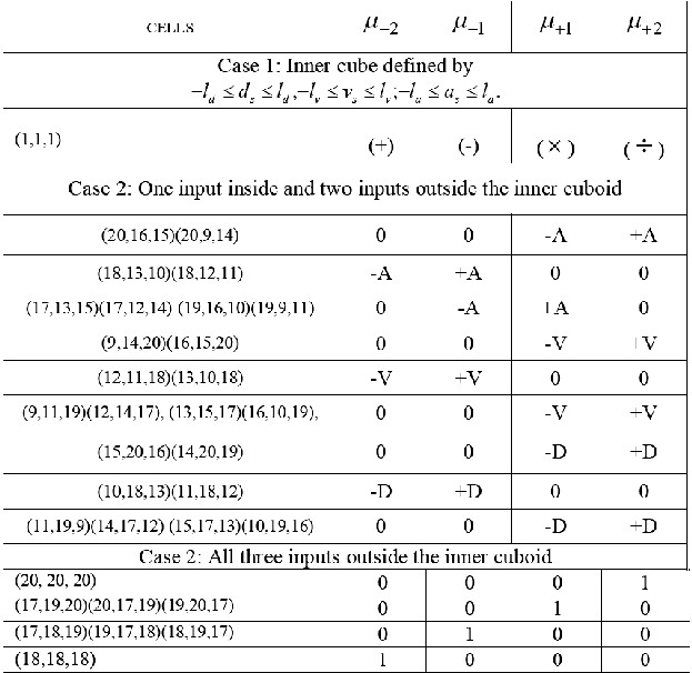
(+): (-D)(-V)(-A)![]()
(-): (-D)(-V)(+A)+(-D)(+V)(-A)+(+D)(-V)(-A)
( ): (-D)(+V)(+A)+(+D)(-V)(+A)+(+D)(+V)(-A) ( ): (+D)(+V)(+A)
In this paper, a mathematical model for a fuzzy PID controller has been derived using L-type, Γ-type and ![]() -type fuzzy
-type fuzzy
membership functions, algebraic product triangular norm,
bounded sum triangular co-norm, algebraic product inference
method, modified output membership functions and CoSdefuzzification method. The model obtained is shown to be nonlinear whereas the model (Class I model) in Mohan and Sinha (2006) was indeed a linear model. The (modified) membership functions considered in Fig. 3 could lead to this difference in the end result.
IJSER © 2012
International Journal of Scientific & Engineering Research,Volume 3, Issue 6, June-2012 6
ISSN 2229-5518
[1]: Wang P and Kwok D P (1992), Analysis and synthesis of an intelligent control system based on fuzzy logic and the PID principle, IntellSystEng, 1:157–
171.
[2]: Mizumoto M (1995), Realization of PID controls by fuzzy control methods, Fuzzy Sets Syst, 70:171–182.
[3]: Qiao W Z and Mizumoto M (1996), PID type fuzzy controller and parameters adaptive method, Fuzzy Sets Syst, 78:23–35.
[4]: Misir D, Malki H A and Chen G (1996), Design and analysis of a fuzzy proportional –integral-derivative controller, Fuzzy Sets Syst, 79:297-314.
[5]: Kim J H and Oh S J (2000), A fuzzy PID controller for nonlinear and uncertain system, Soft Comput, Springer Berlin Heidelberg New York,
4:123–129.
[6]: Woo Z W, Chung H Y and Lin J J (2000), A PID type fuzzy controller with self-tuning scaling factors, Fuzzy Sets Syst, 115:321–326.
[7]: Xu J X, Hang C C and Liu C (2000), Parallel structure and tuning of a fuzzy PID controller, Automatica, 36:673–684.
[8]: Golob M (2001), Decomposed fuzzy proportional-integral-derivative controllers, Appl. Soft Computing, 1:201-204.
[9]: Hu B G, Mann G K I and Gosine R G (2001), A systematic study of fuzzy
PID controllers–function-based evaluation approach, IEEE Trans Fuzzy Syst,
9:699–712.
[10]: Guzelkaya M, Eksin I and Yesil E (2003), Self-tuning of PID-type fuzzy logic controller coefficients via relative rate observer, EngApplArtifIntell,
16:227–236.
[11]: Mohan B M and Arpita S (2006), The simplest fuzzy PID controllers:
mathematical models and stability analysis, Soft Computing, 10:961-975.
[12]: Mohan B M and Arpita S. (2008a), Analytical Structures for Fuzzy PID Controllers?, IEEE Trans. Fuzzy Systems, 16:52-60.
[13]: Mohan B M and Arpita S (2008b), Analytical structure and stability analysis of a fuzzy PID controller, Appl. Soft Computing, 8:749-758
IJSER © 2012