International Journal of Scientific & Engineering Research, Volume 3, Issue 6, June-2012 1

ISSN 2229-5518

A Neuroplasticity (Brain Plasticity) Approach to

Use in Artificial Neural Network

Yusuf Perwej , Firoj Parwej

Abstract — you may have heard that the Brain is plas tic. As you know the brain is not made of plas tic, Brain Plasticity also called Neuroplasticity. Brain plasticity is a physical process. Gray matter can actually shrink or thicken neural connections can be forged a nd refined or weakened and severed. Brain Plasticity refers to the brain’s ability to change throughout life. The brain has the amazing ability to reorganize itself by forming new connections among brain cells (neurons). For a long time, it was believed that as we aged, the con nections in the brain became fixed. Research has shown that in fact the brain never stops chang ing through learning. Plasticity is the capacity of the brain to change with learning. Changes associated with learning occur mostly at the level of the connections among neurons. New connections can form and the internal structure of the existing synapses can change but also partially its internal topology, according to either the received external stimuli and the pre existent connection. W e have found this idea can be applied also to the simple Artificial Neural Network. In this pap er we have proposed a new method is presented to adapt dynamically the topology of an Artificial Neural Network using only the information on lea rning set. And als o in this paper we have proposed algorithm has been tested on result relative to the Multilayer Perceptron (MLP) problem.

Index Terms — Learning, Neuroplasticity, Multilayer Perceptron (MLP), Artificial Neural Network (ANN), Neuron, Brain, Synaptic.

1. INTRODUCTION

——————————  ——————————
rtificial Neural Network (ANN) mimics biological information processing mechanisms. They are
typically designed to perform a nonlinear mapping from a set of inputs to a set of outputs. Artificial Neural Network is developed to try to achieve the biological system type of performance using a dense interconnection of simple processing elements analogous to biological neurons.
The Artificial neural network is being applied to a wide variety of automation problems including adaptive control, optimization, medical diagnosis, decision making, as well as information and signal processing, including speech processing. The first significant paper on artificial neural network is generally considered to be that of McCullock and Pitts [1] in 1943. This paper outlined some concepts concerning how biological neurons could be expected to operate. The neuron models proposed were modeled by simple arrangements of hardware that attempted to mimic the performance of the single neural cell.
A multilayer perceptrons are a network of simple neurons called perceptrons. The basic concept of a single perceptron was introduced by Rosenblatt in 1958. The perceptron computes a single output from multiple real-valued inputs by forming a linear combination according to its input weights and then possibly putting the output through some nonlinear activation function. A single perceptron is not very useful because of its limited mapping ability . No

Mr. Yusuf Perwej (M.Tech, MCA) is currently working in Jazan

University, Jazan , Kingdom of Saudi Arabia (KSA).

E-mail : yusufperwej@gmail.com

Mr. Firoj Parwej (MBA (IT), MCA, BIT) is currently working in

Jazan University, Jazan , Kingdom of Saudi Arabia (KSA).

E-mail : firojparwej@gmail.com
matter what activation function is used, the perceptron is only able to represent an oriented ridge-like function. The perceptrons can, however, be used as building blocks of a larger, much more practicable structure. A typical multilayer perceptron (MLP) network consists of a set of source nodes forming the input layer, one or more hidden layers of computation nodes, and an output layer of nodes. The input signal propagates through the network layer-by- layer.
These topologies are very different with found in biological neural system where network are often much less regular. Since the particular problem can be an optimal solution from a network with non regular connection topology, the goals of transforming over size regular connected network into such an optimal non regular network is complete commit to the learning algorithm. The most of learning algorithm are not able to produce a reduce topology by zeroing synaptic weight, they typically produce different structure spreading non vanishing weights all over the network. The effective and efficient result can be poor. In fact if the network is too small the input and output mapping cannot be learned with satisfying accuracy .If the network is too large after long training phase it will be learn correctly but the badly generalize due to learning data over fitting [2]. The over fitting is especially dangerous because it can easily lead to predictions that is far beyond the range of the training data [3].

2. BIOLOGICAL NEURON

IJSER © 2012 http://www.ijser.org

International Journal of Scientific & Engineering Research, Volume 3, Issue 6, June-2012 2

ISSN 2229-5518

The An artificial neural network (or simply a neural network) is a biologically inspired computational model which consists of processing elements (called neurons) and connections among them with coefficients (weights) bound to the connections, which constitute the neuronal structure, and training and recall algorithm attached to the structure. Neural Network is called connectionist models because of the main role of the connections on them. The connection weights are the "memory" of the system. Even though neural Network has similarities to the human brain, they are not meant to model it. They are meant to be useful models for problem-solving and knowledge-engineering in a "humanlike" way. The human brain is much more complex and unfortunately, many of its cognitive functions are still not well known. But the more we learn about the human brain, the better computational models are developed and put to practicable use.
The human brain contains about 1011 neurons participating in perhaps 1015 interconnections over transmission paths. Each of these paths could be a meter longs or more. Neurons share many characteristics with the other cells in the body, but they have unique capabilities for receiving, processing, and transmitting electrochemical signals over the neural pathways that make up the brain's communication system. Figure 1 shows the structure of a neuron.
The neurons are composed of a cellular body, also called the soma, and its one or several branches. According to the traditional definition the branches conducting information into a cell (stimulus) are called dendrites [4] and the branch that conducts information out of the cell (reaction) is called an axon. An activation of a neuron called an action potential is transmitted to other neurons through its axon at the first instance. A signal (spike) emitted from a neuron is characterized by frequency, duration, and amplitude. The interaction among neurons takes place at strictly determined points of contact called synapses. In the region of the synapses, the neurons almost "touch" one another. In a synapse, the two parts can be distinguished first presynaptic membrane, belong to the transmitting neuron, and another postsynaptic membrane, which belong with the receiving neuron. The electric potential on the two sides of the membrane is called the membrane potential. The membrane potential is formed by the diffusion of electrically charged particles. All cells contain a solution rich in potassium salts. At rest, the cellular membrane is 50 to 100 times more permeable to K+ ions than to Na+ ions. Chloride ions (C1-) are also of great importance in the process of information processing in the brain. The brain consists of different types of neurons. They differ in shape (pyramidal, granular, basket etc.) and in their specialized
functions. There is a correlation among the function of a cell and its shape.
The human brain is a complicated communication system . This system transmits messages as electric

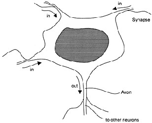
Figure -1 A structure of a neuron. It has many inputs (in) and one output (out). The connections among neurons are realized in the synapses

impulses, which seem always the same, recurring in monotonous succession. A single nerve impulse carries very little information therefore, processing of complex information is only possible by the interaction of groups of many neurons and nerve fibers, which are enormous in number and size. The total length of all neural branching inside the human body comes to about 1014 m. The presence of such a high number of links determines a high level of massive parallelism, which is specific to the brain mechanisms. The human brain as a whole is capable of solving complex problems in a comparatively short time part of a second or several seconds.
The human brain has the ability to learn and to generalize. The information we accumulate as a result of our learning is stored in the synapses in the form of concentrated chemical substances. The brain receives information through its receptors which are [5] connected by dendrites to neurons of the respective part of the cortex (the part of the brain which receives signals from the human sensors). So two of the major processes which occur in the brain from the information processing point of view are learning and recall (generalization). Learning is achieved in the brain through the process of chemical change in synaptic connections. There is a hypothesis which says that the synaptic connections are set genetically in natal life and subsequent development (learning) is due to interactions among the external environments and the genetic program during postnatal life. The learning process in the brain is a

IJSER © 2012 http://www.ijser.org

International Journal of Scientific & Engineering Research, Volume 3, Issue 6, June-2012 3

ISSN 2229-5518

complex mixture of innate constraints and acquired experience. But learning is not only a process of filtering sensory inputs. "Brains actively seek sensory stimuli as raw material from which to create perceptual patterns and replace stimulus-induced activity" [6]. Brains are goal seekers. A brain activity pattern is a drive toward a goal. The activity patterns are spatial and temporal and large patterns of activity are self-organized.

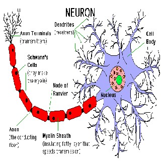
Figure - 2 A structure of a typical biological neuron

The human brain stores pattern of information in an associative mode, that is, as an associative memory. Associative memory is characterized in general by its ability to store patterns, to recall these patterns when only parts of them are given as inputs, for example, part of a face we have seen before, or the tail of a rat. The patterns can be corrupted, for example, an airplane in foggy weather. It has been proved experimentally [7] that part of a region of the human brain called CA3 works as an associative storage and another part (which consists of "mossy" fiber connections) is non associative. Figure 2 shows the structure of a typical biological neuron.
The question of how information is stored in the brain relates to the dilemma of local vs. distributed representation. There is biological evidence that the brain contains parts, areas, and even single neurons that react to specific stimuli or are responsible for particular functions. A neuron, or group of neurons, which represent a certain concept in the brain, is called a grandmother cell. At the same time, there is evidence that the activity of the brain is a collective activity of many neurons working together toward particular patterns, features, functions, tasks, and goals. A chaotic process is, in general, [8] not strictly
repetitive. It does not repeat exactly the same patterns of behaviour, but still certain similarities of patterns can be found over periods of time, not necessarily having the same duration. A chaotic process may be an oscillation among several states, called attractors, which oscillation is not strictly regular. A common oscillation in cortical potential over an entire array of neurons has been recorded [7]. It is beyond the current level of existing knowledge and technology to simulate a human brain in a computer.

3. ARTIFICIAL NEURAL NETWORK

An artificial neural network (or simply a neural network) is a biologically inspired computational model which consists of processing elements (called neurons) and connections among them with coefficients (weights) bound to the connections, which constitute the neuronal structure, and training and recall algorithm attached to the structure. Neural Network is called connectionist models because of the main role of the connections on them. The connection weights are the "memory" of the system. Even though neural network has similarities to the human brain, they are not meant to model it. They are meant to be useful models for problem-solving and knowledge-engineering in a "humanlike" way. The human brain is much more complex and unfortunately, many of its cognitive functions are still not well known. But the more we learn about the human brain, the better computational models are developed and put to practicable use.

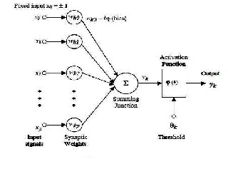
Figure - 3 The Mathematical Model of Artificial Neural

Network

Once modeling an artificial functional model of the biological neuron, we must take into account three basic components. First off, the synapsis of the biological neuron is modeled as weights. Let’s remember that the synapse of the biological neuron is the one which interconnects the neural network and gives the strength of the

IJSER © 2012 http://www.ijser.org

International Journal of Scientific & Engineering Research, Volume 3, Issue 6, June-2012 4

ISSN 2229-5518

connection. For an artificial neuron , the weight is a number , and
represents the synapse. A negative weight reflects an inhibitory connection, while positive values designate excitatory connections. The following components of the model represent the actual activity of the neuron cell. All inputs are summed altogether and modified by the weights. This activity is referred as a linear combination. Finally, an activation function controls the amplitude of the output. Mathematically, this process is described in the Figure 3.

4. NEUROPLASTICITY ( BRAIN PLASTICITY )

Neuroplasticity (Brain Plasticity) is the hottest topic both in science and the public sphere right now. You may have heard that the brain is plastic. As you know the brain is not made of plastic Neuroplasticity (brain plasticity) refers to the brain’s ability to change throughout life. The brain has the amazing ability to reorganize itself by forming new con- nections among brain cells (neurons). Neuroplasticity also known as [9] cortical re-mapping refers to the ability of the human brain to change as a result of one's experience. For the past four hundred years this new thinking was inconceivable because mainstream medicine and science believed that brain anatomy was fixed. The conventional knowledge was that after infancy the brain cannot really change itself and was fully developed, only at the old age when the brain starts the long process of decline was it believed to change. This theory of the unchanging brain put people with mental and emotional problems under a lot of limitations. It basically meant that if you had the problems like an eating disorder, you approximately have to suffer from a life of taking drugs and being sick. But now, [11] we have important data from psychoanalytical therapies and neuroscience that shows that when patients come in with their brains in certain states of miss wiring (mental states) then after undertaking psychological (neuroplastic) interventions their brains can be rewired without drugs or surgeries. This proves that neuroplastic therapy is every bit as biological as the use of drugs and even more precise at times because it is targeted.

5. THE PROPOSED NEUROPLASTICITY PRUNING APPROACH USING ARTIFICIAL NEURAL NETWORK

The brain consists of nerve cells in other words neurons and glial cells which are interconnected and learning may happen through changes in the strength of the connections by adding or removing connections and by the formation of new cells. Neuroplasticity ( brain plasticity ) relates to
learning by adding or removing connections , or adding cells [10] . For
example, each time we learn a new dance step, it reflects a change in our physical brains new "wires" (neural pathways) that gives instructions to our bodies on how to perform the step. Each time we forget someone's name, it also reflects brain changes "wires" that once connected to the memory have been degraded, or even severed. As these examples show, changes in the brain can result in improved skills (a new dance step) or a weakening of skills (a forgotten name).These changes are both structural and functional. Structural plasticity means the brain can
• Grow new neurons (neurogenesis)
• Alter the distribution of where neurons are located
(somatotopic mapping)
• Promote new, extensive synaptic Network in response to
virtually any stimulus and regardless of age, condition, or type of experience.
The functional implication of neuroplasticity is that the brain is always learning. The facts that the brain is actively growing, changing, and learning throughout life can have a positive influence on memory and cognition, emotion, motor learning virtually anything that effects quality of life. The possible draw nears to produce network with correct topology. First start with a small network [11] and grow additional synapses (neurons) until the desired behavior is reached. Another start with a large network and prune off synapses (neuron) until the desired behavior is maintained. The first apprize although it could be efficient since most of the job is performed on the network of small size can be difficult to realize and control to reach network topologies which are optimal in some sense [12]. In single non optimal procedure to add neurons to a multilayer perceptron is reported. The second apprize is much more studied and consists of finding a subset of network synaptic weights that when the set is zero and lead to the smallest increase of an error mensuration in the output. In this paper some contemplation on the biological network plasticity, an idea is introduced to developed a procedure for varying the network topology by simply pruning off connection with an initial over dimensioned fully connected network.
The purpose of synaptic pruning is believed to be to remove unnecessary neuronal structures from the brain as the human brain develops the need to understand more complex structures become much more pertinent, and simpler associations formed in the childhood are thought to be replaced by complex structures [13]. Despite the fact it has several connotations with regulation of cognitive childhood development pruning is thought to be a process of removing neurons which may have become damaged or degraded to further improve the "networking" capacity for

IJSER © 2012 http://www.ijser.org

International Journal of Scientific & Engineering Research, Volume 3, Issue 6, June-2012 5

ISSN 2229-5518

a particular area of the brain. Furthermore, it has been stipulated that the mechanism doesn't only work in regard to development and reparation, but also as a means of continuously maintaining more efficient brain function by removing neurons by their synaptic efficiency [14] The during critical period the network change not only the synaptic strengths of connection but also partly its internal topology .These changes are driven by either the received external stimuli and the preexistence connection layout. We have found that this idea can be applied also to simple artificial neural network. By using only the external stimuli in other words input and output patterns and the network knowledge of the synaptic weights it is possible to adopt the network to the problem changing simultaneously the network synapses and the connection topology. A simple procedure to prune off connection from a fully connected network is presented here. No need for a new connection is created although a similar apprize could be followed to derive a procedure to add synapses to the network.
In this paper artificial neural network is considered in which there are input, output and hidden neurons and all possible connections between these units are allowed generally including recursive connection and self feedback connection. According to the authors [15] when training the recursive network is derived then that the error signal as defined by the specialized delta rule, when calculated by the balanced state of the recursive network and applied at the output of the network and allowed to the backpropagate recursively and error signal at each unit for correction the weight in a gradient descend sense. These fully interconnected Networks are found to have often a greater learning capacity and better error features than the corresponding feedforward network. According to biological behavior this measure must be proportional either to the external stimuli and the pre existent synaptic strength below this formula showed.
an average total synaptic strength proportional to the n-th neuron .Where ITn is the total number of inputs to the n-th neuron. A measure of the importance of the synapsis can be obtained by comparing its averaged strength with respect to the total average strength proportional to the neuron which the synapsis belong with. Therefore the synaptic strength Average (SSA) can be defined as follows.
SSAnm = 1000 ânm / an
The learning phase the previous quantities vary until they reach constant values. This thought is used for changing the network topology consists in dynamically removing the all connections which present an SSA lower than a threshold value varies according to a predefined curve. In the next step of the learning phase each neuron [16] the synaptic strength of every connection proportional to the current training pattern is computed and accrued and the end of the training set all the SSA can be computed. These values are compared with a threshold TV(tp) which is a function of the epoch in a way depending on the particular problem. The connections with an SSA lower than the threshold values are pruned off.

6. EXPRIMENTAL RESULTS OF NEUROPLASTICITY USING ARTIFICIAL NEURAL NETWORK

The proposed method has been tested with the Multilayer Preceptron (MLP) model. Always, the SSA is averaged on one learning epoches, although this was seen to be not critical. The threshold functions used in
anm

= (Wnm actm )

tp

ânm =

ITp

tp 1

ITn

anm

tp 2

tp

/ ITp
an =

ânm

m 1

The synaptic strength of the connection of the n-th neuron coming from the m-th neuron and proportional to the tp-th training pattern where Wnm is the synaptic weight of the connection among the n-th and m-th neurons, and acttp is the activation of the m-th neuron similar to the tp-th input pattern. This activity can be averaged overall training set where ITp is the number of the input training patterns. Since each neuron is driven by several different synapses,

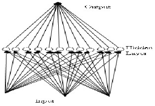
Figure - 4 The Complete Artificial Neural Network Model

these experiments are the Gaussian function
TV (tp) = (q r) -1/2 (s- o / φ) 2
An elemental procedure has been added to the pruning

IJSER © 2012 http://www.ijser.org

International Journal of Scientific & Engineering Research, Volume 3, Issue 6, June-2012 6

ISSN 2229-5518

algorithm which allows in a layer to prune off an entire neuron if it is not connected to any neuron of the upper layer. Where q, o and φ are constant values and the factor
1000 has been removed. We are using artificial neural
network with 3 inputs, 12 hidden neurons and 1 output
have been used to classify 1000 points equally distributed
inside and outside a unit circle on the plane.

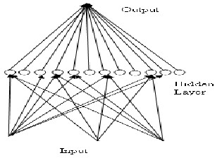
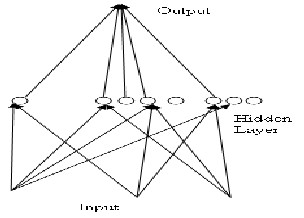
Figure - 5 The Common Topologies Obtained After

Pruning Artificial Neural Network Model

The high output classifies points inside the circle, while the null output classifies points outside it. 100 Network with different, randomly selected initial weights have been generated and used in the experiment. Each network was trained over 3000 epoches using the 1000 points as learning set, Figure 4 shows the original artificial neural network and two common topologies obtained after pruning Artificial Neural Network Model shows Figure 5 and Figure 6.
The values of o and φ parameters are therefore not critical

providing that the network is not disturbed

Figure - 6 The Common Topologies Obtained After

Pruning Artificial Neural Network Model

during the early and late phases of learning. The q value depends also on the size of the network, in other words the number of synapses per neuron and it is not particularly critical. Point out that selecting o and s small allows to rationalize the computational burden since most of the learning is performed on a rationalized network.

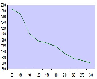
Maximum

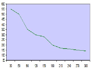
Figure - 7 The graph of the maximum output error vs the number of learning epoches obtained by the figure 3

Artificial Neural Network Model

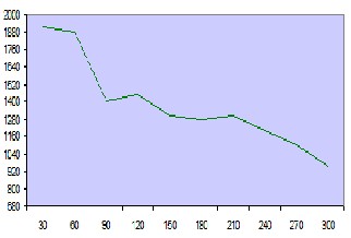
In this paper we are used in 1000 points as learning set, while 4000 points, randomly selected inside the region, and were used as test set Figure 4 and Figure 5. About 66.67% of connections have been pruned off (24/36) and the networks continue to converge. Looking at the maximum error plots Figure 7 and Figure 8 i.e. the maximum of the output error over the whole learning

Maximum

IJSER © 2012 http://www.ijser.org

International Journal of Scientific & Engineering Research, Volume 3, Issue 6, June-2012 7

ISSN 2229-5518

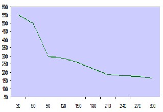
Figure - 8 The graph of the maximum output error vs the number of learning epoches obtained by the figure 4

Artificial Neural Network Model

Mean Square Error (MSE)

Figure - 9 The graph of the Mean Square Error (MSE) vs the number of learning epoches obtained by the figure 3

Artificial Neural Network Model

set versus the training epoch, we can see how, here the pruning phase has the positive effect during the first
period of learning. Figure 9 and Figure 10 report the Mean- Square Error (MSE) at the output, computed over the whole training set, versus the learning epoch, respectively for the complete network Figure 4 and for the pruned network Figure 5 .The pruning period does not disturb the convergence process the smoothness shows of the MSE curve in the Figure 9 case. After many epoches however both Mean Square Error (MSE) and maximum error of the complete networks are often slightly better than those of the pruned network due to the large number of parameters of the first network with respect to the second.

Mean Square Error (MSE)

Figure - 10 The graph of the Mean Square Error (MSE) vs the number of learning epoches obtained by the figure 4

Artificial Neural Network Model

Table - 1 The pruned of 0% training and test set with the maximum output error and MSE obtained from the Network of figure 3

Table - 2 The pruned of 66.67% training and test set with the maximum output error and MSE obtained from the Network of figure 4

The reports of the Table 1 and Table 2 is maximum error and Mean Square Error (MSE) values obtained from the 3
Network after 300 training epoches, using the test set as input. Here the prolixity of the complete network is diminutive the pruned network shows similar or better performance on the test set with respect to the complete network using several synapses reduced to the 33.33% of the original.

7. CODE IN MATLAB

for i = 1:iterat

out = zeros(36,1);

numIn = len (inp(:,1));

for j = 1:numIn

H1 = bias(1,1)*wegt(1,1)

+ inp(j,1)*wegt(1,2)

+ inp(j,2)*wegt(1,3);

x2(1) = sigma(H1);

H2 = bias(1,2)*wegt(2,1)

+ inp(j,1)*wegt(2,2)

+ inp(j,2)*wegt(2,3);

x2(2) = sigma(H2);

H3 = bias(1,3)*wegt(3,1)

+ inp(j,1)*wegt(3,2)

+ inp(j,2)*wegt(3,3);

x2(3) = sigma(H3);

H4 = bias(1,4)*wegt(4,1)

+ inp(j,1)*wegt(4,2)

IJSER © 2012 http://www.ijser.org

+ inp(j,2)*wegt(4,3);

x2(4) = sigma(H4);

H5 = bias(1,5)*wegt(5,1)

+ inp(j,1)*wegt(5,2)

+ inp(j,2)*wegt(5,3);

x2(5) = sigma(H5);

International Journal of Scientific & Engineering Research, Volume 3, Issue 6, June-2012 8

ISSN 2229-5518

H6 = bias(1,6)*wegt(6,1)

+ inp(j,1)*wegt(6,2)

+ inp(j,2)*wegt(6,3);

x2(6) = sigma(H6);

H7 = bias(1,7)*wegt(7,1)

+ inp(j,1)*wegt(7,2)

+ inp(j,2)*wegt(7,3);

x2(7) = sigma(H7);

H8 = bias(1,8)*wegt(8,1)

+ inp(j,1)*wegt(8,2)

+ inp(j,2)*wegt(8,3);

x2(8) = sigma(H8); H9 = bias(1,9)*wegt(9,1)

+ inp(j,1)*wegt(9,2)

+ inp(j,2)*wegt(9,3);

x2(9) = sigma(H9);

H10 = bias(1,10)*wegt(10,1)

+ inp(j,1)*wegt(10,2)

+ inp(j,2)*wegt(10,3);

x2(10) = sigma(H10); H11 = bias(1,11)*wegt(11,1)

+ inp(j,1)*wegt(11,2)

+ inp(j,2)*wegt(11,3);

x2(11) = sigma(H11);

H12 = bias(1,12)*wegt(12,1)

+ inp(j,1)*wegt(12,2)

+ inp(j,2)*wegt(12,3);

x2(12) = sigma(H12);

x3_1 = bias(1,13)*wegt(13,1)

+ x2(1)*wegt(13,2)

+ x2(2)*wegt(13,3);

+ x2(3)*wegt(13,4);

+ x2(4)*wegt(13,5);

+ x2(5)*wegt(13,6);

+ x2(6)*wegt(13,7);

+ x2(7)*wegt(13,8);

+ x2(8)*wegt(13,9);

+ x2(9)*wegt(13,10);

+ x2(10)*wegt(13,11);

+ x2(11)*wegt(13,12);

+ x2(12)*wegt(13,13);

out(j) = sigma(x3_1);

del3_1 = out(j)*(1-out(j))*(output(j)-out(j)); del2_1 = x2(1)*(1-x2(1))*wegt(13,2)*del3_1; del2_2 = x2(2)*(1-x2(2))*wegt(13,3)*del3_1; del2_3 = x2(3)*(1-x2(3))*wegt(13,4)*del3_1; del2_4 = x2(4)*(1-x2(4))*wegt(13,5)*del3_1; del2_5 = x2(5)*(1-x2(5))*wegt(13,6)*del3_1; del2_6 = x2(6)*(1-x2(6))*wegt(13,7)*del3_1; del2_7 = x2(7)*(1-x2(7))*wegt(13,8)*del3_1; del2_8 = x2(8)*(1-x2(8))*wegt(13,9)*del3_1; del2_9 = x2(9)*(1-x2(9))*wegt(13,10)*del3_1; del2_10 = x2(10)*(1-x2(10))*wegt(13,11)*del3_1; del2_11 = x2(11)*(1-x2(11))*wegt(13,12)*del3_1; del2_12 = x2(12)*(1-x2(12))*wegt(13,13)*del3_1; for k = 1:13

wegt(2,k) = wegt(2,k) + coeff*bias(1,2)*del2_2; wegt(3,k) = wegt(3,k) + coeff*bias(1,3)*del2_3; wegt(4,k) = wegt(4,k) + coeff*bias(1,4)*del2_4; wegt(5,k) = wegt(5,k) + coeff*bias(1,5)*del2_5; wegt(6,k) = wegt(6,k) + coeff*bias(1,6)*del2_6; wegt(7,k) = wegt(7,k) + coeff*bias(1,7)*del2_7; wegt(8,k) = wegt(8,k) + coeff*bias(1,8)*del2_8; wegt(9,k) = wegt(9,k) + coeff*bias(1,9)*del2_9; wegt(10,k) = wegt(10,k) + coeff*bias(1,10)*del2_10; wegt(11,k) = wegt(11,k) + coeff*bias(1,11)*del2_11; wegt(12,k) = wegt(12,k) + coeff*bias(1,12)*del2_12; wegt(13,k) = wegt(13,k) + coeff*bias(1,13)*del3_1; else

wegt(1,k) = wegt(1,k) + coeff*inp(j,1)*del2_1; wegt(2,k) = wegt(2,k) + coeff*inp(j,2)*del2_2; wegt(3,k) = wegt(3,k) + coeff*inp(j,3)*del2_3; wegt(4,k) = wegt(4,k) + coeff*inp(j,4)*del2_4; wegt(5,k) = wegt(5,k) + coeff*inp(j,5)*del2_5; wegt(6,k) = wegt(6,k) + coeff*inp(j,6)*del2_6; wegt(7,k) = wegt(7,k) + coeff*inp(j,7)*del2_7; wegt(8,k) = wegt(8,k) + coeff*inp(j,8)*del2_8; wegt(9,k) = wegt(9,k) + coeff*inp(j,9)*del2_9; wegt(10,k) = wegt(10,k) + coeff*inp(j,10)*del2_10; wegt(11,k) = wegt(11,k) + coeff*inp(j,11)*del2_11; wegt(12,k) = wegt(12,k) + coeff*inp(j,12)*del2_12; wegt(13,k) = wegt(13,k) + coeff*x2(k-1)*del3_1;

end

end end

end

8. CONCLUSION

Finally, the brain is a multi layered parallel structure in which is estimated 100 billion nerve cells also called neurons are interconnected and exchange information through neural Network. In the brain, each neuron is connected to thousands of other neurons through synapses. A connected neuron receives input from several other neurons, and when the input weight reaches a threshold value, the neuron propagates an electrical signal that stimulates output through the ignition of a neurotransmitter in other words (input to another neuron). Neurons are to lay constantly down new pathways for neural communication and to rearrange existing ones throughout life, Thereby aiding the processes of learning,

IJSER © 2012 http://www.ijser.org

International Journal of Scientific & Engineering Research, Volume 3, Issue 6, June-2012 9

ISSN 2229-5518

memory, and adaptation through experience. Plasticity relates to learning by adding or removing connections, or adding cells. In this paper we have proposed this method to adapt dynamically the topology of artificial neural Network using the information of the learning set. Although the method eliminates the connection from an initial fully connected network without creating new synapses. In this paper experimental result obtained with the multilayered artificial neural Network is reported on the show the capabilities of the proposed method. This mechanism is shown to capacitate learning of the Multilayer Perceptron (MLP) problem without the aid of error Backpropagation as well as to increase validity, robustness of learning in the presence of interference and noise.

REFERENCES

[1] McCullock, W.W, Pitts, W. ,―A Logical Calculus of the Ideas Imminent in Nervous Activity‖ , Bulletin of Mathematical Biophysics, vol 5 , pp 115-133, 1943.

[2] M . Smith, ―Neural Network for Statistical Modelling‖ , Boston

International Thomson Computer Press , ISBN 1-850-32842-0,

1996.

[3] E.B. Baum , and D. Haussler , ― What size net gives valid generalization‖ , Neural computation , no. 1 , pp 151-160, 1989.

[4] Pelvig, D P, Pakkenberg, H Stark, AK ,Pakkenberg B., ―Neocortical glial cell numbers in human brains‖. Neurobiology of Aging 29, vol (11), pp 1754 – 176 2, April 2007. PMID 17544173, doi:10.1016/j.neurobiolaging.2007.04.013.

[5] B. Draganski , C. Gaser , V. Busch ,G. Schuierer , U. Bogdahn ,

―Neuroplasticity: changes in grey matter induced by training‖ ,

Nature. 427 , pp 311-312, May 2004.

[6] W. Freeman , and C. Skarda , ―Spatial EEG patterns, non-linear dynamics and perception‖ The neo-Sherringtonian vew, Brain Research Reviews 10 , pp 147-175, 1985.

[7] E. Rolls , and A. Treves , ―Neural Network in the brain involved in memory and recall‖ , In Proceedings of Internatonal Joint Conference on Neural Network, Nagoya, Japan, IEEE, pp 9-14, October 1993.

[8] W. Freeman ,― Simulation of chaotic EEG patterns with a dynamic model of the olfactory system‖ Biological Cybernetics 56 , pp

139-150, 1987.

[9] Shaw, Christopher, McEachern, Jill, eds, ―Toward a theory of neuroplasticity ‖, London, England , Psychology Press. ISBN 9781841690216., 2001.

[10] P. Rakic , ―Neurogenesis in adult primate neocortex: an evaluation of the evidence‖, Nature Reviews Neuroscience 3 (1), pp 65–71 , January 2002. doi:10.1038/nrn700, PMID 11823806.

[11] W. Eberhard, and M. J. ,‖Developmental Plasticit

and Evolution ―, Oxford University Press, USA, 2003.

network‖ , ICS Report 8901, UCSD, 1989.

[13] G. Roth , and U. Dicke ,―Evolution of the brain and Intelligence‖,Trends in Cognitive Sciences 9 (5), pp 250–257, 2005. doi:10.1016/j.tics.2005.03.005, PMID 15866152

[14] Abitz, Damgaard et al , ―Excess of neurons in the human newborn mediodorsal thalamus compared with that of the adult‖ , Oxford, Oxford Journals Cerebral Cortex Advance Access Cerebral Cortex, 11 January 2007. doi:10.1093/cercor/bhl163

[15] F. J. Pineda, ―Recurrent backpropagation and the dynamical approach to adaptive neural computations‖, Neural Computations, no 1, pp 161-172, 1989.

[16] L. Yuille , and D. Geiger , ―The Handbook of Brain Theory and Neural Networks‖ , edited by Arbib M. A. , MIT Press, Cambridge, pp 1056–1060, 1995.

Yusuf Perwej received the M .Tech degree

in Computer Science and Engineering from the C-DAC
(Centre for Development of Advanced Computing) Govt. of India Research & Development Center, Noida (India) in
2007, MCA degree in computer application from the
University of GGSIP, Delhi (India) in 2005 .He is currently the department of Research and development member and
Senior Lecturer in the department of Computer Science & Information System at University of Jazan , Kingdom of Saudi Arabia (KSA) . He has authored a number of different journal and paper. His research interests include Soft Computing, Artificial Neural Network, Machine Learning, Pattern Matching & Recognition, Artificial Intelligence, Image Processing, Fuzzy Logic, Bluetooth and Network. He is a member of IEEE.

[12] T. Ash ,― Dynamic node creation in backpropagation

IJSER © 2012 http://www.ijser.org