Inte rnatio nal Jo urnal o f Sc ie ntific & Eng inee ring Re se arc h Vo lume 3, Issue 3 , Marc h -2012 1
ISSN 2229-5518
A Modified Stage-Stacking Method for Multi- Stage Axial Flow Compressor Calculations
Tonye K. Jack and Robin L. Elder
Abs tract— In this paper an attempt w as made at studying multi-sage axial f low compressor off-design perf ormance based on tw o existing stage stacking correlations – the STEINKE (the Un ited States NASA model – ref erred to as the NASA model), and the HOWELL-CALVERT (the United Kingdom NGTE model – ref ered to as the H-C model). Variable stator stagger setting is incorporated in an existing Cranf ield optimisation model; and the primary objective is to see if improvements in overall compressor perf ormance can be achieved by combining these models. An exhaustive study in multistage axial compressor perf ormance has not been conducted. The authors how ever believe the relationships provide a basis at estimating axial compressor perf ormance. A computer program based on the model w ill be developed.
Co mpressor, Off-Design Perf ormance, Stage Stacking, Variable Stator Stagger
—————————— ——————————
Stage-to-stage analysis method is often adopted in eva- luating and predicting the performance of multistage axial flow compressors from stage loading factor
(ΔTCp/U) and pressure rise coefficient (ψ) versus flow coeffi- cient (Φ) relationships [1]. Key parameters and operational
considerations such as tip clearance, stage, stall, Reynolds Number, losses, and others are often designed and analysed based on certain existing derived analytical and/or experi- mental models. Several models exist. The poser for this re- search effort has been: So many Models! Can Axial Compres- sor Performance be improved by parameters study of combin- ing related aspects of these several Models?
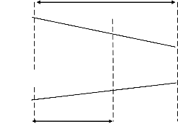
relationship for locating stall point. Because of the stage inte- ractions and mismatches that occur during flow separation, a reference location at entry to the stage with the first stage inlet as datum is used to indicate the stall point. This is effectively saying that since stall is “local”, locating the point of stall could be anywhere after the exit of a stage plus the inlet to the next stage. This is similar to the work of Wassel [4], in which the effective length is indicated by the following relationship:
N entry tofirst stage rotor
![]()
Effective length
The loss model adopted is based on the Wiscelenus [2] model, where, stalling or separation limits is defined based on the stalling coefficient, σ. In the Wiscelenus model, σ, has values of: σ = 0.5, 0.67, 1. The worst case scenario is assumed to occur at the minimum value of σ. This model was also adopted by Lieblein and others [3], in their break-through research work in deriving the NASA diffusion factors.
Based on the model adopted, limiting conditions where set for the stalling flow. Furthermore, critical rotor choke flow condi- tions can be predicted (see Appendix).
Figure (1) shows a simple model that was used to derive a
————————————————
Robin L. Elder, Ph.D, Professor of Turbomachinery Design and Engineer- ing, and former Head of Turbomachinery and Engineering Mechanics De- partment, School of Mechanical Engineering, Cranfield University, Eng-
N 0.5 exit of last stage rotor
Where, N = stage number
This is similar to the present study in which the location of stall is indicated by the following relation:
Stall Point = (Leff - Lx), with the datum at the inlet of the first rotor, and Lx calculated from the point of stall to the exit of last stage rotor.
In arriving at a useful relationship for the stall efficiency based on the H-C model [5], the assumption of stall point indicated by twice the minimum loss value, show that the factor, f = 1. This value indicates that the stall efficiency equals the max i- mum stage efficiency. This also implies that the H -C model applies only at flows above stall i.e. M/Ms≥1. An alternative approach will be a model that arrives at a lower, medium, and upper limiting values for the factor, f. This is a more useful model and shows that the stall efficiency is represented by the product: (sef.ηme). Where, sef is the stall efficiency factor based on the range of values of factor, f, when applied to “(6)” in the Appendix. The lower and upper limits of factor, f , corres- pondd to the stalling or separation limits. It should also be noted that the results arrived at agree with the inception of stall in the H-C correlation.
land. He is currently a Director of PCA Engineers Ltd, a Turbomachinery
Engineering Consultancy.
IJSER © 201 2
Inte rnatio nal Jo urnal o f Sc ie ntific & Eng inee ring Re se arc h 2
ISSN 2229-5518
The Koch-Smith [6] and Lakshiminarayana [7] models where incorporated in accounting for the effect of tip clearance, and other boundary layer effects. A general relationsh ip for com- puting the tip clearance is given based on the Koch -Smith [6] model. At the stage maximum efficiency, the Lakshiminaraya- na [7] model was combined with the H-C [5] model, and pro- vides a useful relationship for estimating the pressure loading, ψ, at maximum stage efficiency.
A simple model was adopted to account for the effect of blockage. This model is based on the geometric annulus area and the overall displacement thickness (Appendix 5).
Effect of stagger setting can be studied with the model, by modifications of inlet and outlet angles, incidence and ca mber angles. However, the model is yet to be fully investigated in this direction and results compared to existing cranfield opti- misation model [8] research that has been conducted in this area.
The effect of Reynolds Number has been built into the present model since the correlation for tip clearance, and displacement thickness calculations was based on the Koch-Smith [6] model. The Reynolds Number range is 2.5 x 10 5-107. Below this region is regarded as laminar.
This paper is not an exhaustive study in the Off-Design per- formance of multistage axial flow compressors. The objective of the exercise has been parameteric studies of the Steinke [9] and Howell-Calvert [5] models to arrive at useful relationships that can be applied in compressor design calculations. This modified method has not been applied to any existing com- pressors, and an example is therefore not presented. The au- thors however believe that the method can further be i m- proved, including the derived equations with additional com- pressor parameters.
This unpublished research effort was conducted at Cranfield University in the autumn months of 1998. The authors wish to thank Cranfield School of Mechanical Engineering for provi d- ing the facilities, particularly their specilised research library materials, and computer laboratories.
P Pressure, N/mm2
T Temperature, K
Pr Pressure Ratio
Tr Temperature Ratio
D Diffusion Factor
deH de Haller Number = 0.72
ks Specific heat Ratio
Cp Specific heat at constant pressure, kJ/kg.K R Gas Constant, J/kg.K
M Mass Flow, kg/s
Mn Mach number
a velocity of air, m/s
U Blade speed, m/s
d Rotor diameter, mm s space, mm
c chord, mm
Cploss Profile loss coefficient
Re Reynolds Number
ML Minimum loss
N Speed, rpm
A Annulus area, m2
B Blockage factor
t Tip clearance, mm
q Relative temperature to relative flow
Leff Effective length, mm
L Length in axial direction, mm h Blade height, mm
W Work input
i incidence angle n A factor
f A factor
sef Stall efficiency factor
V Flow Velocity. m/s
F Parameters
Subscripts and addition notation
a Axial
s indicates condition at stall cr Critical flow condition
me Point of maximum efficiency
1 Inlet of compressor
x Measured axially from compressor inlet stall location
NASA National Aeronautics and Space Administration
NGTE National Gas Turbine Establishment
Greek Symbols
ρ Density, kg/m3
η Stage efficiency
η’ Stage efficiency without endwall losses
λ Work done factor
δ* Displacement thickness, mm
δFθ Tangential force thicjness, mm
κ A constant
ζ Stagger angle
θ Comber angle
βm Mean flow angle α2 Air angle at outlet α1 Air angle at inlet
σ Stalling coefficient factor
Ψ Pressure coefficient
IJSER © 201 2
Inte rnatio nal Jo urnal o f Sc ie ntific & Eng inee ring Re se arc h 3
ISSN 2229-5518
Φ Flow coefficient
τ parameter
τw Shear Stress in wall
χ constant
Λ Degree of reaction
Δ Difference or change in parameter
[1] M.D. Doyle and S.L. Dixon, “The Stacking of Compressor Stage Cha- racteristics to Give an Overall Compressor Performance”, The Aero- nautical Quarterly, pp. 349-367, Nov. 1962.
[2] Wiscelenus, Fluid Mechanics of Turbomachinery Belmont, Calif.:
McGraw-Hill, 1947.
![]()
Va
U
C pT1 Tr 1
![]()
U 2
![]()
k 1
(1) (2)
[3] S. Lieblein, F.C. Schwenk, R.L. Broderick, “Diffusion Factor for Estimating
Pr 1
Losses and Limiting Blade Loadings in Axial Flow Compressor Blade Ele-
ments” , NACA-RME53D01, 1953.
[4] A.B. Wassel, “Reynolds number Effects in Axial Flow Compressor”,
Tr 1
(3)
ASME-67-WA/GT-2
[5] A.R. Howell and W. T. Calvert, “A New Stage Stacking Technique for Axial Flow Performance Technique,” ASME J. of Engr. For Power, vol. 2, no. 4, pp. 193 -218, Apr. 1978.
[6] C.C. Koch, and L.H. Smith, “Loss Sources and their ma gnitudes in
Axial Flow Compressors,” ASME J. of Engr. For Power, vol. 2, no. 4, pp. 193-218, July 1976.
[7] B. Lakshiminarayana, “End Wall and Profile Losses in low Speed
Axial Compressors”, ASME-85-GT-174, pp. 22-31
[8] Jinju-Sun, “Modeling Variable Stator Stagger Settings in Multistage
Axial Flow Compressors,” PhD dissertation, School of Mechanical En-
In this case: (M/Ms<1), and the required relationship is:
n
gineering, Cranfield University., Cranfield, England, 1998.
M
F
1 F
M
(4)
![]()
![]()
7
s s
![]()
7
s
[9] R.J. Steinke, “A Computer Code for Predicting Multistage Axial
Compressor Performance by Meanline Stage Stacking Method”,
NASA-TP-2020, 1982
[10] R. Bullock, and I. Johnsen, eds. “Aerodynamic Design of Axial Flow Com-
pressors,” eds., NASA-SP 36, 1965.
[11] H. Cohen, G.F.C. Rogers, H.I.H. Saravanamutoo, Gas Turbine Theory
Belmont, Calif.: Longman, pp. 123-135, 1996.
[12] J.E. Crouse, “Computer Program for Aerodynamic and Blading Design for
multistage Axial Flow Compressors”., NASA-TP 1946, 1981.
[13] N.A. Cumpsty, Compressor Aerodynamicsas Belmont, Calif.: Longman, pp. 123-135, 1996.
In this case: (M/Ms≥1), and the required relationship is:
q 12
![]()
[14] E.M. Greitzer, “Surge & Rotating Stall in Axial Flow Compressor,” J. 1 F3
(5)
of Engr. For Power, vol. 2, no. 4, pp. 193-218, Apr. 1976.
[15] W.T. Howell, “Stability of Multistage Axial Compressors,” Aero
Quarterly, vol. 2, no. 4, pp. 193-218, Apr. 1964.
[16] A.B. Mckenzie, Axial Flow Fans and Compressors, 1997.
[17] H. Pearson, and T. Bowmer, “Surging of Axial Compressors,” Aero
Quarterly, vol. 2, no. 4, pp. 19 5-210, 1949.
[18] R.G. Willoh, and K. Selder “Multistage Compressor Simulation A p-
me q
Where,
![]()
T
me
plied to the Prediction of Axial Flow Instabilities”, NASA -TM X-
q T
(5a)
1880, 1969
[19] T.K. Jack, and R.L. Elder, “Decoding the NGTE/Calvert Axial Flow Compressor Program,” International Journal of Science and Engineering Research. Submitted for publication. (Pending publication)
![]()
me
Or
IJSER © 201 2
q tan1 tan 2
(5b)
Inte rnatio nal Jo urnal o f Sc ie ntific & Eng inee ring Re se arc h 4
ISSN 2229-5518
q≈1, at maximum stage efficiency
U 2 1.96T 2 k 2
(12a)
5F f
12
s
6
Substituting for U in ―(2)‖ of the STEINKE model re-
me
1 1 23 f
12
(6)
sults in the following relationships:
F6
425 250
![]()
500
(6a)
T 1
k 25C r
s p 49T
(13)
Because the H-C model was based on a diameter of
Tr 1
400 mm rotor stage, for other stages, an efficiency
![]()
k s 25R 49T 1
(14)
scaling factor given by ―(7)‖ is applied:
1
400
![]()
(7)
d
![]()
s a
tan1 tan 2
p
(15)
A correlation based on a change in temperature is used to express critical flow conditions and given by;
2
After substitution through eliminating, U and Cp from
―(15)‖, the following modified relationship, ―(16)‖ is ob-
tained for the temperature rise:
adjustedT
0.01
![]()
![]()
1 F
(8)
ks
1 V 2
(16)
![]()
originalT
4
Ts ![]()
tan 1 tan 2
1.01M
cr
ks R
corrected 1 1 original
(9)
Further substitution, results in a temperature rise, giv- en by ―(17)‖ in terms of the Mach number, Mn:
2 T
Ts M n
k s 1tan 1 tan 2
(17)
![]()
F4 0.008 rotor
(10)
![]()
ks 1
ks
From H-C model, at conditions other than air at k=
1.4, the following relationship applies:
![]()
25R Pr
49T k
s
1
1
(18)
k s
U
![]()
1.4T
(11)
The next couple of steps show methods for arriving at the stage efficiency relationships and other compres- sor parameters. It should be noted that major steps in
their derivations have been omitted and only the key
U 1.4Tks
(12)
and final steps are shown.
IJSER © 201 2
Inte rnatio nal Jo urnal o f Sc ie ntific & Eng inee ring Re se arc h 5
ISSN 2229-5518
1 2 2 i
(23)
Factor f, in ―(6)‖ from the H-C model is given by:
V
At maximum stage efficiency, F3=0, and η=ηme
stall : w
f V
(19)
V
max .eff . : w
V
For turbomachines, the following relationships can be applied in estimating the displacement thickness, δ*:
The values for factor f, are, 0.5; 0.67; and 1 – based on the modified Wiscelenus loss relationship.
On assumption of 50 % reaction, the stall efficiency
as a function of the maximum stage efficiency is given
by:
For f = 0.5, ηs = 0.8ηme
* 1 V .dA
Blockage B 1 1 * / A
The wall shear stress is:
w 0.003V
(24)
(25)
For f = 0.67, ηs = 0.829ηme
And the static pressure difference is given by,
P 80
V
(26)
For f = 1, ηs = ηme
![]()
w *
Substituting and rearranging, we have,
P 0.24
2 V .
(27)
![]()
From ―(5)‖ of the H-C model,
![]()
V
* W mU Vw
![]()
me
1
F q 12
![]()
q
(20)
―(27)‖ can be rewritten to obtain ―(28)‖
Substituting for q, gives ―(21)‖:
P
![]()
0.72 2
V
![]()
(28)
![]()
F tan
tan
12
![]()
me
1 3 1 2
tan1 tan 2
(21)
1 V
3 *
―(21)‖ can be reduced to the form of ―(22)‖ by trigo- nometric adjustment,
Where
F tan
1 12
3 1 2
me
1
tan1
2
1
(22)
ML
P
![]()
12 V
(28a)
IJSER © 201 2
Inte rnatio nal Jo urnal o f Sc ie ntific & Eng inee ring Re se arc h 6
ISSN 2229-5518
P A L T M
![]()
1 1 eff x s
4 deH
(33)
x *
3 ML
A T P
From ―(4)‖,
x 1 x x
M
F
1 F
n
M
(29)
Effective Stall Point = (Lef f – Lx) from datum.
![]()
![]()
7
s s
![]()
7
s
With F7 typically taken as 0.5, the following relation- ship for factor n is obtained,
From the H-C model, the change in efficiency is given by:
2
6280N
![]()
![]()
![]()
Log
Log M
31
(34)
s
n
![]()
Log M
s
M s
(30)
Or
7k sT
' 6280N
31
![]()
7k T
(34a)
Using figure (1), and the conditions for stall, the fol- lowing limiting condition applies:
s
Where, η’ is the stage efficiency of the free stream without end-wall loss and given by the modified Koch- Smith relationship:
25 ML
M
25 ML
(31)
![]()
![]()
24
x
![]()
![]()
6
x
![]()
1 *
'
h
(35)
![]()
1 F
Again using figure (1), and noting that,
Upon substitution, and noting that, (δFθ/t) = 1.5, the tip
clearance, t, is given by the relationship:
![]()
PV cons tan t
(32)
![]()
t h
![]()
![]()
![]()
3
1 1
![]()
2
18840N 1 *
(36)
1
3
7k T
h
T
s
Or By combining the H-C model and the Lakshimina- rayana loss estimating relationship,i.e.
P1 A1 Leff
![]()
T1
![]()
Px Ax Lx
Tx
(32a)
![]()
0.7t
![]()
t
![]()
12
h 1 10
c
(37)
cos m
cos m
Where,
IJSER © 201 2
Inte rnatio nal Jo urnal o f Sc ie ntific & Eng inee ring Re se arc h 7
ISSN 2229-5518
The following simplified relationship for the tip clear- ance-to-chord ratio, (t/c), is obtained as:
Where,
![]()
18840N
![]()
1 h
t 1 3
7k T
![]()
1 3t
![]()
0.001 cos m
(38)
s
![]()
2h
(44)
c
This can be used to estimate the loading coefficient at maximum efficiency.
1
And
1
2 1 i
From ―(27)‖, the work input into the stage can be writ- ten as,
![]()
F4 0.008
1
2
Leff
(45)
2
P V
*
x
w a 2 1
![]()
![]()
0.24V 2
W mU.V
mUV
tan
tan
(39)
Or Datum 1-1
P V
U
![]()
![]()
2 0.48 * mVa
![]()
2 tan 2 1 1
0.5 V
0.5V
(40)
x
1 Lx 2
P V
U
Fig.1: A simplified compressor model
![]()
![]()
![]()
Loss 0.5V 2 0.48 * m 0.5sV 2 Va tan 2 i 1
(41)
Where, κ, is a constant given by,
cos cos
2 1 2 1
cos 2 1 cos 2 1
(42)
By combining the H-C and Koch-Smith models, the critical flow is given by,
M cr
![]()
M
![]()
1.01 F 0.01
(43)
4
IJSER © 201 2