Inte rnatio nal Jo urnal o f Sc ie ntific & Eng inee ring Re se arc h Vo lume 3, Issue 2, Fe bruary -2012 1
ISSN 2229-5518
A Framework for Spatial Data Mining
B. Uppalaiah, Dr. N. Subhash Chandra, A. Srinivas, Prof. T. Ajay Kumar and M,Suman
Abs tract: Our framew ork f or spatial data mining heavily depend on the eff icient processing of neighborhood relations since the neighbo rs of many objects have to be investigated in a single run of a typical algorithm. Theref ore, providing general concepts f or neighborhoo d relations as w ell as an eff icient implementation of these concepts w ill allow a tight integration of spatial data mining algorithms w ith a spatial database management system. This w ill speed up both, the development and the execution of spatial data mining a lgorithms. In this paper, w e def in e neighborhood graphs and paths and a small set of database primitives f or their manipulat ion. We show that typical spatial data mining algorith ms are w ell sup- ported by the proposed basic operations. For f inding signif icant spatial patterns, only certain classes of paths “ leading aw ay” from a starting ob- ject are relevant. We discuss f ilters allow ing only such neighborhood paths w hich w ill signif icantly reduce the search space f or spatial data mining algorithms. Furthermore, w e introduce neighborhood indices to speed up the processing of our database primitives. We imple men ted the data- base primitives on top of a commercial spatial database management system. The eff ectiveness and eff iciency of the proposed appr oach was evaluated by using an analytical cost model and an extensive experimental study on a geographic database.
Inde x Terms— Database Primitives for Spatial Data Min ing, Algorithms f or Spatial Data Mining, Ef f icient DBMS Support Based on
Neighborhood Indices.
—————————— ——————————
1 INTRODUCTION
he computerization of many business and government transactions and the advances in scientific data collection tools provide us with a huge and continuously increasing amount of data. This explosive growth of databases has far
outpaced the human ability to interpret this data, creating an urgent need for new techniques and tools that support the human in transforming the data into useful information and knowledge. Knowledge discovery in databases (KDD) has been defined as the non-trivial process of discovering valid, novel, and potentially useful, and ultimately understandable
patterns from data [FPS 96]. The process of KDD is interactive and iterative, involving several steps such as the following ones:
• Selection: selecting a subset of all attributes and a subset of all data from which the knowledge should be discovered.
•Data reduction: using dimensionality reduction or transforma- tion techniques to reduce the effective number of attributes to be considered.
• Data mining: the application of appropriate algorithms that,
under acceptable computational efficiency limitations, pro- duce a particular enumeration of pa tterns over the data.
• Evaluation: interpreting and evaluating the discovered pa t- terns with respect to their usefulness in the given application.
Spatial Database Systems (SDBS) (see [Gue 94] for an overview) are database systems for the management of spatial data. To find implicit regularities, rules or patterns hidden in large spa- tial databases, e.g. for geo-marketing, traffic control or envi- ronmental studies, spatial data mining algorithms are very important (see [KHA 96] for an overview of spatial data min- ing).
Most existing data mining algorithms run on separate and specially prepared files, but integrating them with a database management system (DBMS) has the following advantages. Re- dundant storage and potential inconsistencies can be avoided. Furthermore, commercial database systems offer various in- dex structures to support different types of database queries. This functionality can be used without extra implementation
effort to speed-up the execution of data mining algorithms (which, in general, have to perform many database queries). Similar to the relational standard language SQL, the use of standard primitives will speed-up the development of new data mining algorithms and will also make them more porta- ble.
In this paper, we introduce a set of database primitives for mining in spatial databases. [AIS 93] follows a similar ap- proach for mining in relational databases. Our database primi- tives are based on the concept of neighborhood relations since attributes of the neighbors of some object of interest may have an influence on the object itself. The proposed primitives are sufficient to express most of the algorithms for spatial data mining from the literature. We present techniques for efficient- ly supporting these primitives by a DBMS.
The rest of the paper is organized as follows. Section 2 intro- duces our database primitives for spatial data mining. In sec- tion 3, we review spatial data mining algori thms and demon- strate how they can be expressed by using the proposed primi- tives. Section 4 presents methods of efficiently supporting our database primitives by existing DBMSs. Section 5 summarizes the contributions and discusses several issues for future re- search.
2 D ATABAS E PRIMITIV ES FOR SPATIAL D ATAMINING
In this section, we introduce a small set of database primitives for spatial data mining (see [EKS 97] for a first sketch). The major difference between mining in relational databases and mining in spatial databases is that attributes of the neighbors of some object of interest may have an influence on the object itself. Therefore, our database primitives are based on the con- cept of spatial neighborhood relations.
2.1 Neighborhood Relations
The mutual influence between two objects depends on factors such as the topology, the distance or the direction between the
IJSER © 201 2
http :// www.ijser.org
Inte rnatio nal Jo urnal o f Sc ie ntific & Eng inee ring Re se arc h Vo lume 3, Issue 2, Fe bruary -2012 2
ISSN 2229-5518
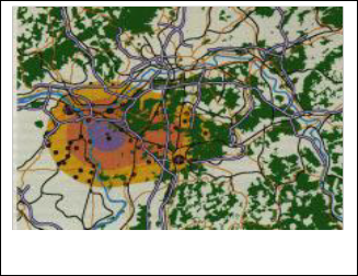
objects. For instance, a new industrial plant may pollute its neighborhood depending on the distance and on the major direction of the wind. Figure 1 depicts a map used in the as- sessment of a possible location for a new industrial plant. The map shows three regions with different degrees of pollution (indicated by the different colors) caused by the planned plant. Furthermore, the influenced objects such as communities and forests are depicted.
Figure 1. Regions of pollution around a planned industrial plant
[BF 91]
In this section, we introduce three basic types of spatial rela- tions: topological, distance and direction relations which are binary relations, i.e. relations between pairs of objects. S patial objects may be either points or spatially extended objects such as lines, polygons or polyhedrons. Spatially extended objects may be represented by a set of points at its surface, e.g. by the edges of a polygon (vector representation) or by the poin ts contained in the object, e.g. the pixels of an object in a raster image (raster representation). Therefore, we use sets of points as a generic representation of spatial objects. In general, the points p = (p1, p2, . . ., pd) are elements of a d-dimensional Euc- lidean vector space called Points. In the following, however, we restrict the presentation to the 2 -dimensional case, al- though, all of the introduced notions can easily be applied to higher dimensions d. Spatial objects O are represented by a Set
off points, i.e. O ∈ 2Points set off points, For a point p = (px, py), px
and py denote the coordinates of p in the first and the second
dimension. ∆x (O):= max {|ox - px| | o, p ∈ O} is called the x- extension of O and ∆y (O):= max {|oy - py| | o, p ∈ O} the y-
extension of O.
Topological relations are those relations which are invariant un- der topological transformations, i.e. they are preserved if both objects are rotated, translated or scaled simultaneously. The formal definitions are based on the boundaries, interiors and complements of the two related objects.
Definition 1: (topological relations) The topological relations between two objects A and B are derived from the nine inter- sections of the interiors, the boundaries and the complements
of A and B with each other. The relations are: A disjoint B, A meets B, A overlaps B, A equals B, A covers B, A covered-by B, A contains B, A inside B. A formal definintion can be found in [Ege 91].
Distance relations are those relations comparing the distance of
two objects with a given constant using one of the arithmetic operators. The distance dist between two objects, i.e. sets of points, can then simply be defined by the minimum distance between their points.
Definition 2: (distance relations) Let dist be a distance func-
tion, let σ be one of the arithmetic predicates <, > or = , let c be
a real number and let O1 andO2 be spatial objects, i.e. O1,O2 ∈
2Points. Then a distance relation A distances σc B holds iff dist (O1,
O2) σc.
In the following, we define 2 -dimensional direction relations
and we will use their geographic names. For dimensions d > 2, the number of different direction relations increases but the underlying concepts are still the same.
To define direction relations O2 R O1, we distinguish between the source object O1 and the destination object O2 of the direction relation R. There are several possibilities to define direction relations depending on the number of points they consi der in the source and the destination object. We define the direction relation of two spatially extended objects using one represen t- ative point rep (O1) of the source object O1 and all points of the destination object O2. The representative point of a source ob- ject may, e.g., be the center o f the object. This representative point is used as the origin of a virtual coordinate system and its quadrants define the directions.
Definition 3: (direction relations) Let rep (A) be a representa- tive point in the source object A.
- B northeast A holds, iff b ∈B: bx ≥³ rep(A)x by ³ rep(A)y
southeast, southwest and northwest are defined analo
gously.
- B north A holds, iff b B: by ³ rep (A) y
south, west, east are defined analogously.
- B any_direction A is defined to be TRUE for all A, B.
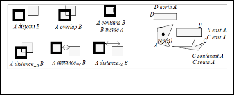
Figure 2 illustrates some of the topological, distance and direc- tion relations using 2D polygons.
Figure 2. Illustration of the direction relations
Obviously, for each pair of spatial objects at least one of the direction relations holds but the direction relation between
IJSER © 201 2
http :// www.ijser.org
Inte rnatio nal Jo urnal o f Sc ie ntific & Eng inee ring Re se arc h Vo lume 3, Issue 2, Fe bruary -2012 3
ISSN 2229-5518
two objects may not be unique. Only the special relations northwest, northeast, southwest and southeast are mutually ex- clusive (if we exclude objects with holes, objects with a co- dimension greater than 0, and separations). However, if con- sidering only these special directions there may be pairs of objects for which none of these direction relations hold, e.g. if some points of B are northeast of A and some points of B are northwest of A. On the other hand, all the direction relations are partially ordered by a specialization relation (simply given by set inclusion) such that the smallest direction relation for two objects A and B is uniquely determined. We call this smal- lest direction relation for two objects A and B the exact direction relation of A and B.
Topological, distance and direction relations may be combined by the logical operators (and) as well as (or) to express a complex neighborhood relation.
Definition 4: (complex neighborhood relations) If r1 and r2 are neighborhood relations, then r1 r2 and r1 r2 are also neighborhood relations - called complex neighborhood relations.
2.2 Neighborhood Graph s and Their Operations
Based on the neighborhood relations, we introduce the con- cepts of neighborhood graphs and neighborhood paths and some basic operations for their manipulation.
Definition 5: (neighborhood graphs and paths) Let neighbor be a neighborhood relation and DB 2Points be a database of ob- jects.
a) A neighborhood graph DB = (N, E) is a graph with the set of nodes N which we identify with the objects o DB and
the set of edges E N N where two nodes n1 and n2 N are connected via some edge of E iff neighbor(n1,n2) holds. Let n
denote the cardinality of N and let e denote the cardinality of
E. Then, f: = e / n denote the average number of edges of a node, i.e. f is called the “fan out” of the graph.
b) A neighborhood path is a sequence of nodes [n1, n2. . . nk], where neighbor (ni, ni+1) holds for all ni N, 1 i < k. The num- ber k of nodes is called the length of the neighborhood path.
c) A neighborhood path [n1, n2. . . nk] is valid iff i k, j < k: i j
ni nj.
Lemma 1: The expected number of neighborhood paths of length k starting from a given node is f k -1 and the expected number of all neighborhood paths of length k is then n*f k -1.
In the following, we will only create valid neighborhood paths, i.e. paths containing no cycles. Obviously, even the number of valid neighborhood paths may become very large. For the purpose of KDD, however, we are mostly interested in a cer- tain class of paths, i.e. paths which are “leading away” from the starting object in a straightforward sense. We conjecture
that a spatial KDD algorithm using a set of paths which are crossing the space in an arbitrary way, leading forward and backwards and contain cycles will not produce useful patterns (if any will be produced at all). Therefore, in addition to our general restriction to valid paths, the operations on neighbor- hood paths will provide parameters (filters) to further reduce the number of paths actually created.
We will present the signature of the most important opera- tions and a short description of their meaning using the fol- lowing domains: Objects, NRelations (neighborhood rela- tions), Predicates, Integer, NGraphs (neighborhood graphs), NPaths (neighborhood paths ), 2Objects, 2NPaths. We do not define an explicit domain of databases. Instead, we use the domain
2Objects of all subsets of the set of all objects.
We assume the standard operations from relational algebra such as selection, union, intersection and difference to be available for sets of objects and for sets of paths. For instance, the opera- tion selection (db, pred) returns the set of all elements of a da- tabase db satisfying the predicate pred. We introduce the fol- lowing basic operations for neighborhood graphs and paths:
neighbors: NGraphs x Objects x Predicates --> 2Objects extensions: NGraphs x 2NPaths x Integer x Predicates -> 2NPaths paths: 2Objects --> 2NPaths;
objects: 2NPaths --> 2Objects
The operation neighbors (graph, object, pred) returns the set of all objects connected to object via some edge of graph satisfy- ing the conditions expressed by the predicate pred. The addi- tional selection condition pred is used if we want to restrict the investigation explicitly to certain types of neighbors. The definition of the predicate pred may use spatial as well as non- spatial attributes of the objects.
The operation extensions (graph, paths, max, and pred) return the set of all paths extending one of the elements of paths by at most max nodes of graph. All the extended paths must satisfy the predicate pred. Because the number of neighborhood paths may become very large, the operation extension is the most critical operation with respect to efficiency of data mi n- ing algorithms. Therefore, the predicate pred in the operation extensions acts as a filter to restrict the number of paths created using domain knowledge about the relevant paths. Note that the elements of paths are not contained in the result implying that an empty result indicates that none of the ele- ments of paths could be extended.
The operation paths (setOfObjects) creates the set of all paths of length 1 formed by a single element of setOfObjects. The operation objects (setOfPaths) returns the set of all objects as- sociated with at least one of the nodes of one element of se- tOfPaths.
IJSER © 201 2
http :// www.ijser.org
Inte rnatio nal Jo urnal o f Sc ie ntific & Eng inee ring Re se arc h Vo lume 3, Issue 2, Fe bruary -2012 4
ISSN 2229-5518
2.3 Filter Predicates for Neighborhood Path s Neighborhood graphs will in general contain many paths which are irrelevant if not “misleading” for spatial data min-
ing algorithms. For finding significant spatial patterns, we
have to consider only certain classes of paths which are “lea d- ing away” from the starting object in some straightforward sense. Such spatial pa tterns are most often the effect of some kind of influence of an object on other objects in its neighbor- hood. Furthermore, this influence typically decreases or in- creases continuously with increasing or decreasing distance. The task of spatial trend analys is, i.e. finding patterns of sys- tematic change of some non-spatial attributes in the neighbor- hood of certain database objects, can be considered as a typical example. Detecting such trends would be impossible if we do not restrict the pattern space in a wa y that paths changing di- rection in arbitrary ways or containing cycles are eliminated.
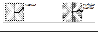
In the following, we discuss two possible filter predicates, star- like and variable-starlike. Other filters may be useful depending on the application.
Definition 6: (filter starlike and filter variable starlike) Let p
= [n1, n2...nk] be a neighborhood path and let reli be the exact direction for ni and ni+1, i.e. ni+1 reli ni holds. The predicates starlike and variable-starlike for paths p are defined as follows: Starlike (p): ( j < k: i > jni+1 reli nireli relj), if k > 1; TRUE, if k=1
variable-starlike(p) :( j < k: i > j: ni+1 reli nireli rel1), if k >
1; TRUE, if k=1.
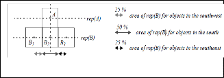
The exact direction relation rel for a source object A and a des- tination object B is not independent from their sizes. If B is smaller than A then rel is likely to be a special relation, if B is larger than A then rel typically is a general direction relation. In the following, we analyze this dependency considering the special but important case of A and B having the same size. Let A be a source object and B be a destination object satisfy- ing A intersect B and B south A. Then, there are three groups of such objects B as depicted in figure 4.
Figure 4. Objects B w ith “ B south of A and B intersects A”
All objects of the middle group B2 fulfill the exact direction relation B2 south A. For the objects of the two outer groups, B1 and B3, the exact direction relation is one of the special rela- tions, i.e. B1 southwest A and B3 southeast A. Assuming a uni- form distribution of the representative points of the B objects and assuming that B intersects A holds, the exact direction relation of the B objects is distributed as follows: 25% south- west, 25% southeast, 50% south. Generalizing this observation, we find that each of the four generalized (specialized) direc- tions is the exact direction relation for 1 6 f (1 12) f out of the f neighbors of some source object. Figure 5 illustrates the distribution of the exact direction relations of the B objects.
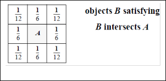
Figure 3. Illustration of two different filter predicates
The filter starlike requires that, when extending a path p, the exact “final” direction relj of p cannot be generalized. For in- stance, a path with “final” direction northeast can only be ex- tended by a node of an edge with exact direction northeast but not by an edge with exact direction north.
The variable-starlike filter is less restrictive than the starlike fil- ter. It requires only that, when extending a path p with a node nk+1, the edge e = (nk, nk+1) has to fulfill at least the exact “in i- tial” direction rel1 of p. Note that relj rel1 holds if a filter (star- like or variable-starlike) is used for each extension starting from length 1. For instance, a neighborhood path with “intial” d i- rection north can be extended by a node nk+1 if e satisfies the direction north or one of the more special directions northeast or northwest. Figure 3 illustrates the neighborhood paths for the filters starlike and variable-starlike when extending the paths from a given starting object.
Figure 5. Distribution of the exact direction relations
Under the above assumptions, we can calculate the number of all starlike neighborhood paths of a certain length l for a given fanout f of the neighborhood graph. The following lemma gives the order of the number of these paths for f = 6 and f =
12.
Lemma 2: Let A be a spatial object and let l be an integer. Let intersects be chosen as the neighborhood relation. If the repre- sentative points of all spatial objects are uniformly distributed and if they have the same x and y, then the number of all starlike neighborhood paths with source A having a length of at most l is O(2l) for f = 12 and O(l) for f = 6.
Lemma 2 allows us to estimate the number of neighborhood paths created when using the filter starlike. The assumptions of
IJSER © 201 2
http :// www.ijser.org
Inte rnatio nal Jo urnal o f Sc ie ntific & Eng inee ring Re se arc h Vo lume 3, Issue 2, Fe bruary -2012 5
ISSN 2229-5518
this lemma may seem to be too restrictive for real applications. Note, however, that intersects is a very natural neighborhood relation for spatially extended objects. To evaluate the as- sumptions of uniform distribution of the representative points of the spatial objects and of the same size of these objects, we conducted a set of experiments to compare the expected num- bers of neighborhood paths with the actual number of paths created on a real database.
A geographic database on Bavaria was used for this experi- mental evaluation. The database contains the ATKIS 500 data [Atk 96] and the Bavarian part of the statistical data obtained by the German census of 1987. Also included are spatial ob- jects representing natural object like mountains or rivers and infrastructure such as highways or railroads. The total number of spatial objects in the database is n = 6,924 and the database size is 57.4 MB.
The average number f of edges of a node plays a crucial role in lemma 2. This lemma calculates the number of starlike neigh- borhood paths for values of f = 6 and f = 12. Therefore, we created a different neighborhood graph for each of these f val- ues from the same geographic database by using the neigh- borhood relations distance a and distance b. The distances a and b were set such that the resulting f value was 6 and 12 re- spectively, that is the total number of edges e was e = 6 *
n and e = 12 * n respectively. In our test database, we found f
6 for the neighborhood relation intersect implying that the
above distance a was close to 0. We selected typical commun i- ties from the geographic database as source objects according to the following criteria. The communities should be located sufficiently far enough from the Bavarian border so that neighborhood paths with a length of at least 5 can be created. There should be a balanced mix of small and a large communi- ty (in terms of their area) since the number of actual neighbors of a community is correlated to its area.
We created all neighborhood paths as well as the starlike neighborhood paths with a maximum length of up to 5 for each of the selected sources. Table 1 reports the results for f = 6
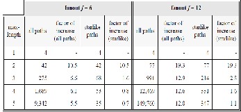
Table 1: Numbers of neighborhood paths
and for f = 12. The table shows the results depending on the parameter maximum length. The largest value of maximum
length was only 5 due to the very large number of all neigh- borhood paths and the corresponding large runtime for creat- ing them. Note that the numbers presented in the columns “all paths“and “starlike paths“ do only count the number of paths having a length of exactly the specified max-length, i.e. they do not count the shorter paths. The columns “factor of i ncrease” give the quotient of the number of paths in the current row and the number of paths in the previous row (i.e. for the pre- vious value of max-length).
We find that for f = 6 the number of all neighborhood paths (starting from the same source) with a length of at most max- length is O(6max-length) and the number of the starlike neighbor- hood paths only grows approximately linear with increasing max-length - as stated by lemma 2. For f = 12 the number of all neighborhood paths with a length of at most max-length is O (12max-length) as we can expect from the lemma. However, the number of the starlike neighborhood paths is significantly less than the stated value O (2max-length). This deviation from lemma
2 can be explained as follows. The lemma assumes the same
size of the spatial objects. However, small destination objects are more likely to fulfil the filter sta rlike than large destination objects implying that the size of objects on starlike neighbor- hood paths tends to decrease. Thus, the factor of increase de- creases significantly because in general small objects have less neighbors than large objects. Note that lemma 2 nevertheless yields an upper bound for the number of starlike neighbor- hood paths created.
The factors of increase, listed in table 1, provide some interes t- ing insights. The factors of increase are approximately as stated by lemma 2. However, we observe that these factors are exceptionally large for max-length = 2, i.e. when comparing the paths for max-length = 1 and maxlength = 2. The reason is that the filter starlike does not yield any restrictions for the exten- sion of paths with length 1 since these paths do not yet have a characteristic direction. Therefore, the factor of increase for max-length = 2 is the same for all paths as for the sta rlike paths.
3 ALGORITHMS FOR SPATIAL DATAM INING
To support our claim that the expressivity of our spatial data mining primitives is adequate, we demonstrate how typical spatial data mining algorithms can be integrated with a spatial DBMS by using the database primitves introduced in section
2.
3.1 Spatial Clustering
Clustering is the task of grouping the objects of a database into meaningful subclasses (that is, clusters) so that the members of a cluster are as similar as possible whereas the members of different clusters differ as much as possible from each other. Applications of clustering in spatial databases are, e.g., the detection of seismic faults by grouping the entries of an earth- quake catalog or the creation of thematic maps in geographic information systems by clustering feature spaces.
IJSER © 201 2
http :// www.ijser.org
Inte rnatio nal Jo urnal o f Sc ie ntific & Eng inee ring Re se arc h Vo lume 3, Issue 2, Fe bruary -2012 6
ISSN 2229-5518
Different types of spatial clustering algorithms have been pro- posed, e.g. k-medoid clustering algorithms such as CLARANS [NH 94]. This is an example of a global custering algorithm (where a change of a single database object may infl uence all clusters) which cannot make use of our database primitives in a natural way. On the other hand, the basic idea of a single scan algorithm is to group neighboring objects of the database into clusters based on a local cluster condition performing only one scan through the database. Single scan clustering algorithms are efficient if the retrieval of the neighborhood of an object can be efficiently performed by the SDBS. Note that local clus- ter conditions are well supported by our database primitives, in particular by the neighbors operation on an appropriate neighborhood graph. The a lgorithmic schema of single scan clustering is depicted in figure 6.
Different cluster conditions yield different n otions of a cluster and different clustering algorithms. For example, GDBSCAN (Generalized Density Based Spatial Clustering of Applications

with Noise) [SEKX 98] relies on a density-based notion of clus- ters. The key idea of a densitybased cluster is that for each point of a cluster its Eps-neighborhood for some given Eps > 0 has to contain at least a minimum number of points, i.e. the “density” in the Eps-neighborhood of points has to exceed some threshold. This idea of “density-based clusters” can be generalized in two important ways. First, any notion of a neighborhood can be used instead of an Eps-neighborhood if the definition of the neighborhood is based on a binary predi- cate which is symmetric and reflexive. Second, instead of simply counting the objects in a neighborhood of an object other measures to define the “cardinality” of that neighbor- hood can be used as well. Whereas a distance-based neighbor- hood is a natural notion of a neighborhood for point objects, it may be more appropriate to use topological relations such as intersects or meets to cluster spatially extended objects such as a set of polygons of largely differing sizes. See [SEKX 98] for a detailed discussion of suitable neighborhood relations for dif- ferent applications.
3.2 Spatial Characterization
The task of characterization is to find a compact description for a selected subset of the database. In this section, we discuss the task of characterization in the context of spatial databases and review two relevant methods.
Extending the general concept of association rules, [KH 95] introduces spatial association rules which describe associations between objects based on spatial neighborhood relations. For instance, a user may want to discover the spatial associ ations of towns in British Columbia with roads, waters, mines or boundaries having some specified support and confidence. Then, the following spatial association rule may be discov- ered:
X DB Y DB: is-a(X, town) close-to(X, Y) is-a(Y,
water) (80%)
This rule states that 80% of the selected towns are close to wa- ter, i.e. the rule characterizes towns in British Columbia as generally being close to some lake, river etc.
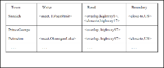
The algorithm presented in [KH 95] to find spatial association rules consists of 5 steps. Step 2 (coarse spatial computation) and step 4 (refined spatial computation) involve spatial as- pects of the objects and are briefly examined in the following. Step 2 computes spatial joins of the object type to be characte- rized (such as town) with each of the other specified object types (such as water, road, boundary or mine) using a neigh- borhood relation (such as close-to). For each of the candidates obtained from step 2 (and which passed an additional fi lter- step 3), the exact spatial relation, for example overlap, is deter- mined in step 4. Finally, a relation such as the one depicted in figure 7 results which is the input for the final step of rule generation. It is easy to see that the spatial steps 2 and 4 of this algorithm can be well supported by the neighbors operation on a suitable neighborhood graph.
SingleScanClustering (Database db; NRelation rel)
set Graph to create_NGraph (db,rel); initialize a set CurrentObjects as empty; for each node O in g do
if O is not yet member of some cluster then
create a new cluster C;
insert O into CurrentObjects;
while CurrentObjects not empty do
remove the first element of CurrentObjects as O;
set Neighbors to neighbors(Graph, O, TRUE);
if Neighbors satisfy the cluster condition do
add O to cluster C;
add Neighbors to CurrentObjects;
end SingleScanClustering;
Figure 6. Schema of single scan clustering algorithms
Figure 7. Input f or the step of rule generation [KH 95]
[EFKS 98] introduces the following definition of spatial chara c- terization with respect to a database and a set of target objects which is a subset of the given database. A spatial characteriza- tion is a description of the spatial and non -spatial properties which are typical for the target objects but not for the whole database. The relative frequencies of the non-spatial attribute values and the relative frequencies of the different object types are used as the interesting properties. For instance, different object types in a geographic database are communities, moun-
IJSER © 201 2
http :// www.ijser.org
Inte rnatio nal Jo urnal o f Sc ie ntific & Eng inee ring Re se arc h Vo lume 3, Issue 2, Fe bruary -2012 7
ISSN 2229-5518
tains, lakes, highways, railroads etc. To obtain a spatial charac- terization, not only the properties of the target objects, but also the properties of their neighbors (up to a given maximum number of edges in the relevant neighborhood graph) are con- sidered.
A spatial characterization rule of the form target p1 (n1, freq- fac1) ... pk (nk, freq- fack) means that for the set of all targets extended by ni neighbors, the property pi is freq-faci times more (or less) frequent than in the database. The characterization algorithm usually starts with a small set of target objects, se- lected for instance by a condition on some non -spatial attribute(s) such as “rate of retired people = HIGH” (see figure
8, left). Then, the algorithms expands regions around the tar- get objects, simultaneously selecting those a ttributes of the regions for which the distribution of values differs significant- ly from the distribution in the whole database (figure 8, right).
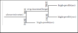
the decision tree, the neighbors of target objects are not consi- dered individually. Instead, so-called buffers are created around the target objects and the nonspatial attribute values are aggregated over all objects contained in the buffer. For instance, in the case of shopping malls a buffer may represent the area where its customers live or work. The size of the buf- fer yielding the maximum information gain is chosen and this size is applied to compute the aggregates for all relevant attributes. Figure 9 depicts an example of a spatial decision tree classifying stores as having a high or low profit.
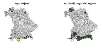
Figure 9. Spatial decision tree [KHS 98]
Whereas the nearest neighbor cannot be directly expressed by our neighborhood relations, it would be possible to extend our set of neighborhood relation accordingly. The proposed data- base primitives are, however, sufficient to express the creation of buffers for spatial classification.
Fig. 8. Characterizing w rt. high rate of retired people [EFKS 98]
In the last step of the algorithm, the following characterization rule is generated describing the target regions. Note that this rule lists not only some non -spatial attributes but also the neighborhood of mountains (after three extensions) as signifi- cant for the characterization of the target regions:
community has high rate of retired people apartments per building = very low (0, 9.1) rate of foreigners = very low (0, 8.9)
rate of academics = medium (0, 6.3)
average size of enterprises = very low (0, 5.8)
object type = mountain (3, 4.1)
Obviously, this algorithm is well suited for support by the
proposed database primitives.
3.3 Spatial Classi fication
The task of classification is to assign an object to a class from a given set of classes based on the attribute values of this object. In spatial classification the attribute values of neighborin g ob- jects are also considered.
The algorithm presented in [KHS 98] works as follows: The relevant attributes are extracted by comparing the attribute values of the target objects with the attribute values of their nearest neighbors. The determination of relevant attributes is based on the concepts of the nearest hit (the nearest neighbor belonging to the same class) and the nearest miss (the nearest neighbor belonging to a different class). In the construction of
3.4 Spatial Trend Detection
A spatial trend has been defined as a regular change of one or more non-spatial attributes when moving away from a given start object o [EFKS 98]. Neighborhood paths starting from o are used to model the movement and a regression analysis is performed on the respective attribute values for the objects of a neighborhood path to describe the regularity of change. For the regression, the distance from o is the independent variable and the difference of the attribute values are the dependent variable(s) for the regression. The correlation of the observed attribute values with the values predicted by the regression function yields a measure of confidence for the discovered trend.
Global as well as local trends are possible. The existence of a global trend for a start object o indicates that if considering all objects on all paths starting from o the values for the specified attribute(s) in general tend to increase (decrease) with increas- ing distance. Figure 10 (left) depicts the result of algorithm global-trend for the attribute “average rent” and the city of Regensburg as a start object. Algorithm local-trends detects single paths starting from an object o and having a certain trend. The paths starting from o may show different pattern of change, e.g., some trends may be positive while the others may be negative. Figure 10 (right) illustrates this case for the attribute “average rent” and the city of Regensburg as a start object.
IJSER © 201 2
http :// www.ijser.org
Inte rnatio nal Jo urnal o f Sc ie ntific & Eng inee ring Re se arc h Vo lume 3, Issue 2, Fe bruary -2012 8
ISSN 2229-5518
Figure 10. Spatial trends of the“ average rent” starting f rom the city of Regensburg
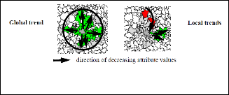
The algorithms for spatial trend detection are naturally su p- ported by our paths and extensions operation.
4 E FFICENT DBMS S UPPORT B AS ED ON
NEIGHBORHOOD INDICES
Typically, spatial index structures, e.g. R -trees [Gut 84], are used in an SDBMS to speed up the processing of queries such as region queries or nearest neighbor queries [Gue 94]. Note that our default implementation of the neighbors operations uses an R-tree. If the spatial objects are fairly complex, howev- er, retrieving the neighbors of some object this way is still very time consuming due to the complexity of the evaluation of neighborhood relations on such objects. Furthermore, when creating all neighborhood paths with a given source object, a very large number of neighbors operations has to be per- formed. Finally, many SDBS are rather static since there are not many updates on objects such as geographic maps or pro- teins. Therefore, materializing the relevant neighborhood graphs and avoiding to access the spatial objects themselves may be worthwhile. This is the idea of the neighborhood in- dices.
4.1 Neighborhood Indice s
In this section, we review related work on join indices and then we introduce our concept of neighborhood indices. The idea of a (relational) join index [Val 87] is to maintain a pre- computed structure containing all pairs of tuples from the two input relations satisfying some join predicate. [Val 87] shows how such indices can be used by a query optimizer to speed - up the processing of join operations. The join index is imple- mented as a binary relation. [Rot 91] introduced the concept
of spatial join indices as a materialization of a spatial join with the goal of speeding up spatial query processing. Given two sets of vertices V1 and V2 and a set of edges E, an abstract join index is defined as the bipartite graph (V1, V2, E). [Rot 91] de-
scribes an algorithm to generate a spatial join index from a
[LH 92] refines the concept of spatial join indices. The el e- ments of the Vi represent objects instead of page regions. A distance associated join index consists of tuples of the form (ob- ject1,object2,distance(object1,object2)) for each pair of database objects. This join index can be used to support not only queries concerning a single neighborhood relation but it is applicable to a large number of queries. Since a distance ass ociated join index requires O(n2) space for a database of n objects, a hierar- chical version is also proposed. These indices assume a spatial concept hierarchy of objects. A hierarchical distance associated join index has one entry only for pairs of objects contained in the same object of the next higher level of the hierarchy. For instance, only pairs of cities in the same state or pairs of hous- es in the same city are represented by an index entry. This ap- proach significantly reduces the space requirements but also prevents its application for spatial data mining if a spatial con- cept hierarchy is either not available or not relevant for the task of mining. For example, in a geographic information sys- tem there may be a spatial concept hierarchy of districts > communities > etc. but the influence of communities to their neighborhood is not restricted to communities of the same district. Consequently, we cannot rely on such hierarchies - representing a political viewpoint - for the purposee of sup- porting spatial data mining.
Our concept of neighborhood indices is related to that of the dis- tance associated join indices with the following new contribu- tions:
• A specified maximum distance restricts the pairs of objects represented in a neighborhood index.
• For each of the different types of neighborhood rela- tions (that is distance, direction, and topological relations), the concrete relation of the pair of objects is stored.
In the following, we introduce neighborhood indices more formally.
Definition 7: neighborhood index
Let DB be a set of spatial objects and let max and dist be real numbers. Let D be a direction relation and T be a topological relation. Then the neighborhood index for DB with maximum
distance max, denoted by I max , is defined as follows:
DB
I max
= {(O1, O2, dist, D, T) | O1, O2 DB, O1 distance=dist O2
grid file. In this case, the elements of the Vi represent the page
regions, that is the sets of cells of the directory mapped to the
same data page. E contains an edge for each pair of vertices from V1 and V2 where the corresponding page regions have an e-overlap for some e specified by the database administrator. Furthermore, an algorithm is presented for updating the join index on updates of the underlying grid files. [Rot 91] does not discuss the physical design of spatial join indices.
dist max O2 D O1 O1 T O2}.
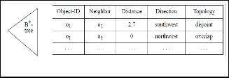
A simple implementation of a neighborhood index using a B+- tree on the key attribute Object-ID is illustrated in figure 11.
IJSER © 201 2
http :// www.ijser.org
Inte rnatio nal Jo urnal o f Sc ie ntific & Eng inee ring Re se arc h Vo lume 3, Issue 2, Fe bruary -2012 9
ISSN 2229-5518
c if r is the relation distance<c or distance=c
if r is a direction, the relation distance> or disjoint
Min(c-distance (r1), c-distance (r2)) if r=r1 r2
Max(c-distance (r1),c-distance(r2)) if r=r1 r2
Figure 11. Sample Neighborhood Index
A neighborhood index supports not only one but a set of neighborhood graphs. We call a neighborhood index applicable
A neighborhood index with a maximum distance of max is applicable for a neighborhood graph with relation r if the criti- cal distance of r is not larger than max. This is the contents of lemma 4.
for a given neighborhood graph if the index contains an entry for each of the edges of the graph. To find the neighborhood
Lemma 4: Let G r
be a neighborhood graph and let I DB be
indices applicable for some neighborhood graph, we introduce the notion of the critical distance of a neighborhood relation r. intuitively, the critical distance of a neighborhood relation r is
a neighborhood index.
If max c-distance(r), then I DB is applicable for DB .
max G r
the maximum possible distance for a pair of objects O1 and O2
satisfying O1 r O2. The following definitions introduce these
Obviously, if two neighborhood indices
DB and DB DB
with
notions formally.
c1 < c2 are available and applicable, using I c 1
is more effi-
DB
Definition 8: applicable neighborhood index
Let GDBr be a neighborhood graph and let I DBmax be a neigh-
DB DB
cient because in general it has less entries than I c 2 . The smal-
lest applicable neighborhood index for some neighborhood graph
is the applicable neighborhood index with the smallest critical
distance.
borhood index. I max is applicable for G r
iff (O1 DB, O2 DB) O1r O2 (O1, O2, dist, D, T)
DB
max
In figure 12, we sketch the algorithm for processing the neigh- bors operation which makes use of the smallest applicable
Definition 9: critical distance of a neighborhood relation
Let r be a neighborhood relation and let denote the set of the real numbers. Let 2Points denote the set of all spatial objects.

neighborhood index. If there is no applicable neighborhood index, then the standard approach of using some spatial index structure is followed.
DB
The critical distance of r, denoted as c-distance(r), is defined as
neighbors (graph G r
, object o, predicate pred)
follows:
select as I the smallest applicable neighbor
DB
r
min(D )if D is non empty
hood index for
; // Index Selection
c-distance(r) =
Otherw ise
if such I exists then // Filter Step
use the neighborhood index I to retrieve as
with the set D defined as:
Dd O1 O2 2PointsO1rO2 O1distance = dist O2) dist
d)}
The following lemma allows to calculate the critical distance for any neighborhood relation. The critical distance is calcu- lated recursively along the composition of a neighborhood relation.
Lemma 3: The following equation holds for the critical dis- tance of a neighborhood relation r:
candidates the set of objects c
having an entry (o,c,dist, D, T) in I
else use the spatial index for DB to retrieve as
candidates
the set of objects c satisfying o r c;
initialize an empty set of neighbors;
// Re finement Step
for each c in candidates do if o r c and pred(c) then
add c to neighbors
return neighbors;
Figure 12. Algorithm neighbors
0
C-distance(r) =
mi n(c di s tan ce(r1 ),c di s tan ce(r 2 ))
max(c di s tan ce(r ),c di s tan ce(r ))
0 if r is a-topological relation except disjoint
The first step of algorithm neighbors, the index selection, selects a neighborhood index. The filter step returns a set of candidate objects (which may satisfy the specified neighborhood rela- tion) with a cardinality significa ntly smaller than the database size. In the last step, the refinement step, for all these candidates the neighborhood relation as well as the additional predicate
IJSER © 201 2
http :// www.ijser.org
Inte rnatio nal Jo urnal o f Sc ie ntific & Eng inee ring Re se arc h Vo lume 3, Issue 2, Fe bruary -2012 10
ISSN 2229-5518
pred are evaluated and all objects passing this test are returned as the resulting neighbors.
To implement the extensions operation, we perform a depth- first search. Thus, a path buffer of size O(max-length) is suffi- cient to store the intermediate results. On the other hand, a breadthfirst search would require a much larger buffer size since it begins creating all paths before finishing the first one. To retrieve the nodes for potential extensions of a candidate path, the neighbors operations is used indicating that the effi- ciency of this operation is crucial. Figure 13 presents the algo- rithm for the extensions operation in pseudo-code notation.

However, the spatial index structure assumed to be available for d supports this retrieval.
Insert-object (database d, object o)
set maximum to the maximum distance of the largest
neighborhood index I d derived from d; retrieve as neighborhood all objects n from d satisfy ing by dist (n, o) maximum using the spatial index structure associated with d;
for each element neighbor of neighborhood do
calculate distance as dist(neighbor,o);
calculate direction as the direction relation of neigh bor and o;
To create a neighborhood index
DB
max
, a spatial join on DB
calculate reverse-direction as the direction relation of
o and neighbor;
with respect to the neighborhood relation O1distance = dist (O2
dist max) is performed. A spatial join can be efficiently
processed by using a spatial index structure, see e.g. [BKSS
94]. For each pair of objects returned by the spatial join, we
then have to determine the exact distance, the direction rela- tion and the topological relation. The resulting tuples of the form (O1, O2, Distance, Direction, Topology) are stored in a rela- tion which is indexed by a B-tree on the attribute O1.
Updates of a database, i.e. insertions or deletions of spatial objects, require updates of the derived neighborhood indices.

Fortunately, the update of a neighborhood index I max is re
extensions(graph g, list of paths p, integer max-length, filter f)
initialize an empty list extensions;
initialize the list of path-candidates to the list p;
while path-candidates is not empty do
remove the first element of path-candidates as
cand;
if length of cand < max-length then
set o to last node of cand;
call neighbors(g,o, TRUE) obtaining the set
neighborhood;
for each element neighbor of neighborhood do
create an extension ext of cand by adding neigh bor as the last node;
if ext is valid and ext satisfies the filter f then
add ext to extensions;
add ext at the head of the list path-candidates;
return path-candidates;
Figure 13. Algorithm extensions
stricted to the neighborhood of the respective object defined by the neighborhood relation A distance< max B. This neighbor- hood can be efficiently retrieved by using either a neighbor- hood index (in case of a deletion) or by using a spatial index structure (in case of an insertion). As an example, we discuss insertions of a new spatial object o to a database of spatial ob- jects d. The retrieval of the relevant neighbors of o is not sup- ported by any neighborhood index since o is a new object.
calculate topology as the topological relation of
neighbor and o;
calculate reverse-topology as the topological relation
of o and neighbor;
for each neighborhood index I max derived from d do if distance max then
insert the entry (neighbor, o, distance, direction,
topology) into I max ;
insert the entry (o, neighbor, distance, reverse-
direction, reverse-topology) into I max ;
Figure 14. Algorithm insert-object
Note that there may be several neighborhood indices derived from the same database d and that all relevant ones have to be updated to include an entry for each of the neighbors of o. Figure 14 presents the algorithm insert-object in pseudo-code notation. In each of the relevant neighborhood indices, two entries have to be inserted for each pair (o,neighbor). Recall that the direction relations and the topological relations are not symmetric so that the relation r has to be determined for o r neighbor as well as for neighbor r o.
4.2 Co st Model
A cost model is developed to predict the cost of performing a neighbors operation with and without a neighborhood index. For database algorithms, usually the number of page accesses is chosen as the cost measure. However, the amount of CPU time required for evaluating a neighborhood relation on spa- tially extended objects such as polygons may become very large so that we model both, the I/O time and the CPU time for an operation. We use tpage, i.e. the execution time of a page access, and tfloat, i.e. the execution time of a floating point com- parison, as the units for I/O time and CPU time, respectively.
In table 2, we define the parameters of the cost model and list typical values for each of them. The system overhead s in- cludes client-server communication and the overhead induced by several SQL queries for retrieving the relevant neighbor- hood index and the minimum bounding box of a polygon (ne-
IJSER © 201 2
http :// www.ijser.org
Inte rnatio nal Jo urnal o f Sc ie ntific & Eng inee ring Re se arc h Vo lume 3, Issue 2, Fe bruary -2012 11
ISSN 2229-5518
cessary for the access of the R-tree). pindex and pdata denote the probability that a requested index page and data page, respec- tively, have to be read from disk according to the buffering strategy.
Table 3 shows the cost for the three steps of processing a neighbors operation with and without a neighborhood index. In the R-tree, there is one entry for each of the n nodes of the neighborhood graph whereas the B+-tree stores one entry for each of the f * n edges. We assume that the number of R-tree
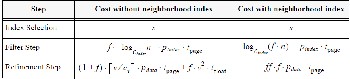
Table 3: Cost model for the neighbors operation
paths to be followed is proportional to the number of neigh- boring objects, i.e. proportional to f. A spatial object with v vertices requires v/cv data pages. We assume a distance rela- tion as neighborhood relation requiring v2 floating point com- parisons. When using a neighborhood index, the filter step returns ff * f candidates. The refinement step has to access their index entries but does not have to access the vertices of the candidates since the refinement test can be directly performed by using the attributes Distance, Direction and Topology of the index entries. This test involves a constant, i.e. independent of v, number of floating point comparisons and requires no page accesses such that its cost can be neglected.
4.3 Experimental Results
We implemented the database primitives on top of the com- mercial DBMS Illustra [Ill 97] using its 2D spatial data blade which provides R-trees. A geographic database of Bavaria was used for an experimental performance evaluation and valida- tion of the cost model. This database represents the Bavarian communities with one spatial attribute (polygon) and 52 non- spatial attributes (such as average rent or rate of unemploy- ment). All experiments were run on HP9000/715 (50MHz) workstations under HP-UX 10.10.
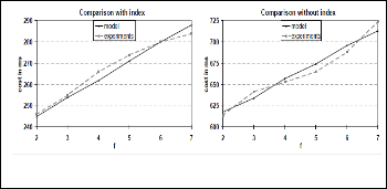
Figure 15. Co mparison of cost model versus experimental r esults
The first set of experiments compared the performance pre- dicted by our cost models with the experimental performance
when varying the parameters n, f and v. The results show that our cost model is able to predict the performance reasonably well. For instance, figure 15 depicts the results for n = 2,000, v
= 35 and varying values for f.
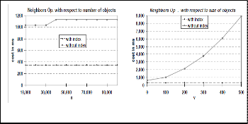
We used our cost model to compare the performance of the neighbors operation with and without neighborhood index for combinations of parameter values which we could not eva- luate experimentally with our database. Figure 16 depicts the results (1) for f = 10, v = 100 and varying n and (2) for n =
100,000, f = 10 and varying v. These results demonstrate a sig- nificant speed-up for the neighbors operation with compared to without neighborhood index. In particular, the neighbor- hood index is very efficient for complex spatial objects, i.e. for large values of v which is typical, e.g., for geographic informa- tion systems.
The next set of experiments analyzed the system overhead which is rather large for a single neighbors operation. This overhead, however, can be reduced when calling multiple correlated
Figure 16. Co mparison w ith and w ithout neighborhood index

Table 2: Parameters of the cost model
neighbors operations issued by one extensions operation, since the client-server communication, the retrieval of the relevant neighborhood index etc. is necessary only once for the whole extensions operation and not for each of the neighbors opera-
IJSER © 201 2
http :// www.ijser.org
Inte rnatio nal Jo urnal o f Sc ie ntific & Eng inee ring Re se arc h Vo lume 3, Issue 2, Fe bruary -2012 12
ISSN 2229-5518
tions. In our experiments, we found that the system overhead was typically reduced by 50%, e.g. from 211 to 100 ms.
To conclude, when using neighborhood indices we obtain a significant speed-up for the neighbors operation. This opera- tion is most crucial to the efficient DBMS support of the data- base primitives since the implementation of the operations for extending neighborhood paths is based on the neighbors op- eration. The speed-up grows strongly with increasing number of vertices of the spatial objects. There is a large system over- head induced by the DBMS which is significantly reduced when considering sets of neighbors operations issued from the same extensions operation.
5 C ONCLUSION
In this chapter, we introduced a framework for spatial data mining which is based on the concepts of neighbourhood graphs and paths. A small set of basic operations on these graphs and paths were defined as database primitives for spa- tial data mining. Furthermore, techniques to efficiently sup- port the database primitives by a commercial DBMS were pre- sented. In the following sections, we covered the main tasks of spatial data mining: spatial clustering, spatial characterization, spatial trend detection and spa tial classification. For each of these tasks, we presented algorithms as well as prototypical applications in domains such as the earth sciences and geo- graphy. Thus, we demonstrated the practical i mpact of these algorithms of spatial data mining.
The following issues indicate interesting directions for future research. The database primitives were implemented on top of the commercial DBMS Illustra. Since the system overhead i m- posed by this DBMS is rather large, techniques of improving the efficiency should be investigated. For example, techniques for processing sets of related neighbours operations which pro- vide more information to the DBMS can be used to improve the overall efficiency of mining algorithms using the database primitives.
In some spatial databases the dimension of time plays an im- portant role: the history of the relevant part of the world is stored for the purpose of analysis, for example raster images of the same area of the surface of the earth taken at different times. Data mining in such spatio-temporal databases is a promising area of future research. For example, geograp hers may be interested in learning spatio-temporal rules describing the process of growth of urban landuse.
ACKNOWLEDGM ENT
We thank International Journal of Scientific & Engineering Research (IJSER). Also we thanks to Holy Mary Institute of Technology and Science (HITS), India, A.P, Hyderabad for finding and supporting this research.
REFERENCES
[AIS 93] Agrawal R., Imielinski T., Swami A.: “Database Mining: A Perfor- mance Perspective”, IEEE Transactions on Knowledge and Data Engineer- ing, Vol. 5, No. 6, 1993, pp. 914-925.
[BF 91] Bill, Fritsch: “ Fundamentals of Geograph ical Information Systems: Hardware, Software and Data” (in German), Wichmann Publishing, Heidel- berg, Germany, 1991.
[Ege 91] Egenhofer M. J.: “Reasoning about Binary Topological Relations”, Proc. 2nd Int. Symp. on Large Spatial Databases, Zurich, Switzerland,
1991, pp. 143-160.
[EKS 97] Ester M., Kriegel H.-P., Sander J.: “Spatial Data Mining: A Database Approach”, Proc. 5th Int. Symp. on Large Spatial Databases, Berlin, Ger- many, 1997, pp. 47-66.
[EFKS 98] Ester M., Frommelt A., Kriegel H.-P., Sander J.: “Algorithms for Characterization and Trend Detection in Spatial Databases”, Proc. 4th Int. Conf. on Knowledge Discovery and Data Mining, New York City, NY,
1998, pp. 44-50.
[FPS 96] Fayyad U. M., .J., Piatetsky-Shapiro G., Smyth P.: “From Data Mining to Knowledge Discovery: An Overview” , in: Advances in Knowledge Discovery and Data Mining, AAAI Press, Menlo Park, 1996, pp. 1 - 34.
[Gue 94] Gueting R. H.: “An Introduction to Spatial Database Systems”, Spe- cial Issue on Spatial Database Systems of the VLDB Journal, Vol. 3, No. 4, October 1994.
[Gut 84] Guttman A.: “R-trees: A Dynamic Index Structure for Spatial Search-
ing“, Proc. ACM SIGMOD Int. Conf. on Management of Data, 1984, pp.
47-54.
[Ill 97] Informix Inc.: ”Illustra User’s Guide”, Version 3.3, 1997.
[KH 95] Koperski K. and Han J.: “Discovery of Spatial Association Rules in Geographic Information Databases”, Proc. 4th Int. Symp. on Large Spatial Databases (SSD ‟95), Portland, ME, 1995, pp 47 -66.
[KHA 96] Koperski K., Adhikary J., Han J.: “Knowledge Discovery in Spatial Databases: Progress and Challenges” , Proc. SIGMOD Workshop on Research Issues in Data Mining and Knowledge Discovery, Technical Report 96-08, University of British Columbia, Vancouver, Canada, 1996.
[KHS 98] Koperski K. , Han J., Stefanovic N.: “An Efficient Two-Step Method for Classification of Spatial Data”, Proc. Symposium on Spatial Data Han- dling (SDH „98), Vancouver, Canada, 1998.
[LH 92] Lu W., Han J.: “Distance-Associated Join Indices for Spatial Range
Search”, Proc. 8th Int. Conf. on Data Engineering, Phoenix, AZ, 1992, pp.
284-292.
[NH 94] Ng R. T., Han J.:“Efficient and Effective Clustering Methods for Sp a- tial Data Mining”, Proc. 20th Int. Conf. on Very Large Data Bases, Sa ntiago, Chile, 1994, pp. 144 -155.
[Rot 91] Rotem D.: “Spatial Join Indices”, Proc. 7th Int. Conf. on Data Engi- neering, Kobe, Japan, 1991, pp. 500 -509.
[SEKX 98] Sander J., Ester M., Kriegel H.-P., Xu X.: “Density-Based Cluster- ing in Spatial Databases: A New Algorithm and its Applications”, Data Mining and Knowledge Discovery, an International Journal, Kluwer Academic Publishers, Vol.2, No. 2, 1998.
IJSER © 201 2
http :// www.ijser.org
Inte rnatio nal Jo urnal o f Sc ie ntific & Eng inee ring Re se arc h Vo lume 3, Issue 2, Fe bruary -2012 13
ISSN 2229-5518
[Val 87] Valduriez P.: “ Join Indices“, ACM Transactions on Database Sys- tems, Vol. 12, No. 2, 1987, pp. 218-246.
AUTHORS PROFILE

B. Uppalaiah received Master of Technology (Software Engi- neering) from Aurora‟s Technological and Research Institute (ATRI) Hyderabad in 2010. His research interests include Data Mining, Network Security and Information Security. He is currently working as an Assistant Professor in the department of Computer Science in Holy Mary Institute of Technology and Science (HITS COE), Hyderabad, A. P, India.
Email : bnp.uppalaiah@gmail.com

Dr. N. Subhash Chandra received Ph. D (Computer Science Engineering) & Master of Technology (Computer Science En- gineering) from Jawaharlal Neh ru Technological University Hyderabad. And he is currently working as a Principal and Professor, department of Computer Science in Holy Mary In- stitute of Technology and Science (HITS COE). His research interests include Image Processing, Speech Processing, Data Mining, Network Security and Information Security.
Email : su bhashchandra_n@yahoo.co.in

A. Srinivas received Master of Technology in Computer Science Engineering in 2009. His research interests include Data Mining, Information Security, Software Testing and Software Quality. He is currently working as an Assistant Pro- fessor, department of Computer Science in Holy Mary Insti- tute of Technology and Science (HITS COE), India,
Email : aoola.srinivas@gmail.com

Prof. T. Ajay Kumar currently pursuing Ph. D (Data Mining) in Acharya Nagarjuna University Guntur, and he received Master of Technology in Computer Science Engineering (SE) from Jawaharlal Nehru Technological Univhersity Anantha- pur. He is currently working as a Professor, department of Computer Science in Holy Mary Institute of Technology and Science. His research interests include Data Mining, Network Security, Software Quality Assurance, Software Engineering. Email: ajay_tenali@yahoo.co.in

M. Suman received Master of Engineering from Hindustan University in July 2010 (Computer Science Engineering) from Inistitute of Aeronautical Engineering. And he is currently working as an Assistant Professor, department of Computer Science in Vidya Vikas Institute of Technology. His research interests include Data Mining, Network Security and Wireless Networks, Cloud Computing.
Email : sumanmecse@gmail.com
IJSER © 201 2
http :// www.ijser.org