International Journal of Scientific & Engineering Research, Volume 4, Issue 4, April-2013 400

ISSN 2229-5518

A Comparative Study of Profit Analysis of Two

Reliability Models on a 2-unit PLC System

Dr. Bhupender Parashar, Dr. Nitin Bhardwaj

Abstract - A two-unit PLC system is analysed with two different situations resulting in to two models. In first model two identical units are used in hot standby and no priority regarding operation/ repair is set for any of the units. W hile in the other model two units are used in hot standby on master-slave basis. The slave unit can also fail but generally its failure rate is lower than that of the master unit. Priority is given to the repair of minor fault over the major fault. In other cases of failure, priority for repair is given to the master unit. Also, priority for operation is given to the master unit. For various measures of system effectiveness the expressions are obtained and a comparative study of both the models is done for the profit with respect to various parameters followed by the conclusion.

Index Terms - Relaibility, Semi-markov, Regenerative Point, PLC, Hot Standby, Comparative Study, Profit

——————————  ——————————

1 INTRODUCTION

In the field of reliability engineering, a number of researchers like [1] to [5] have analysed various models under different assumptions and collecting real data. System based on a particular model cannot be considered as best. A model may be better in some situations and may be worse in some other situations when compared with some other models. Keeping this in view, the present study deals with the comparison between two models at a time to see which is better than the other under the stated situations. The comparison is done graphically considering the particular case that the time to repair/replacement are exponential as taken in the concerned models. Graphs are plotted taking the values of rates, costs and probabilities estimated based upon the data collected from an industry. Values of some other rates/costs have been assumed wherever used.
The system is analysed by making use of semi-Markov
processes and regenerative point technique and expressions for
different measures of the system effectiveness are obtained.

2. MODEL - I

2.1 Assumptions

1. Initially one unit is operative and the other is hot standby.
2. Failure times are assumed to have exponential
distribution whereas the other times have general
distributions.
3. There are two types of failure - minor failures (repairable)
and major failures (irreparable).
4. After each repair, the system works as good as new one.
In this model, it is considered that both the operative as well as the standby unit are identical and no particular unit is given any priority for operation/ repair. All failures are repaired by an expert repairman.

2.2 Notations

O - operative unit
hs - hot standby unit
 - constant failure rate of the unit
 - constant failure rate of the hot standby unit
p - probability of minor failure
q1 - probability of minor failure (repairable) q2 - probability of major failure (irreparable) Fre - unit is under repair in case of minor failure
FRe - repair by the repairman is continuing from the previous state
Frep - unit is under replacement in case of major failure FRep - replacement is continuing from the previous state wre - failed unit waiting for repair from the repairman wrep - failed unit waiting for replacement from the
repairman
g1(t), G1(t) - p.d.f. and c.d.f. of repair time of unit having
minor failure
h(t), H(t) - p.d.f. and c.d.f. of replacement time of unit having major failure

w(t) t) - p.d.f. and c.d.f. of waiting time.
- Stieltjes transform

2.3 Transition Probabilities and Mean Sojourn Times

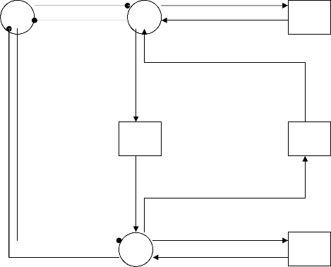
A transition diagram showing the various states of transition of system is shown as in Fig. 1. The epochs of entry into states 0, 1 and 2 are regenerative points and thus these states are regenerative states. The transition probabilities are given below:
p01 = p + q1 ,
p02 = q2 ,
p13 = (p + q1)[1 – g1*()] , p14 = q2[1 – g1*()] ,
p10 = g1*() , p20 = h*() ,
p25 = (p + q1)[1 – h*()] ,

International Journal of Scientific & Engineering Research, Volume 4, Issue 4, April-2013 401

ISSN 2229-5518

p26 = q2[1 – h*()] ,

(3)

The unconditional mean time taken by the system to transit for any regenerative state ‘j’ when it (time) is counted from the

p11

(4)



(p + q1)[1 – g1*()] ,
epoch of entrance into state ‘i’ is mathematically stated as



p12



q2[1 – g1*()] ,

 tdQ (t)

 - q* ' (0)

(5)

(6)



(p + q1)[1 – h*()],
Thus,
mij = 0

ij ij

p22



q2[1 – h*()]
m01 + m02 = 0
By these transition probabilities, it can be verified that p01 + p02 = 1

(3) (4)

m10 + m13 + m14 = 1
m20 + m25 + m26 = 2



p10 + p13 + p14 = 1 = p10 + p11

 p12  G

(5) (6)

m10+m11(3)+m12(4) = 0
1(t) dt = 1 (say)
p20 + p25 + p26 = 1 = p20 + p21

 p 22 

The mean sojourn time (i) in the regenerative state ‘i’ are given by



 H

m20+m21(5)+m22(6) = 0
(t) dt = 2 (say)

0 = λ  α , 1 =

1  g1 (λ )

, 2 =

1  h(λ )

(p+q1) (+) (p+q1) 

0 1 3

(o, hs)

g1(t)

(Fre, o)

g1(t)

(FRe, wre)

h(t)

q2(+)

g1(t)

q2

(FRe, wrep) (p+q1) 

q2

h(t)

(FRep, wre)

(Frep, o)

Fig. 1

h(t)

(FRep, wrep)

Up State

Failed State

 Regeneration Point

International Journal of Scientific & Engineering Research, Volume 4, Issue 4, April-2013 402

ISSN 2229-5518

2.4 Mean Time to System Failure

Regarding the failed state as absorbing states and employing the arguments used for regenerative processes, we have the following recursive relation for i(t) .
where,

lim s BR * (s)

BR0 = s0

N 2

= D1

0(t) = Q01(t) 1(t) + Q02(t) 2(t)
1(t) = Q10(t) 0(t) + Q13(t) + Q14(t)
2(t) = Q20(t) 0(t) + Q25(t) + Q26(t)
Now, taking L.S.T. of the above equations and solving them for
0**(s), the mean time to system failure (MTSF) when the
system starts from the state 0, is
N2 = 1 [p01 p20 + p21(5)] and D1 is already specified.

2.7 Busy Period Analysis of Expert Repairman

(Replacement Time Only)

Using the probabilistic arguments, we have the following recursive relations for BRPi(t) :
BRP0(t) = q01(t) © BRP1(t) + q02(t) © BRP2(t)
BRP1(t) = q11(3)(t) © BRP1(t) + q12(4)(t) ©BRP2(t)+q10(t) ©
BRP0(t)

lim

MTSF = s0
Where

1 - φ**(s) N



s D

BRP2(t) = W2(t) + q21(5)(t) © BRP1(t) + q22(6)(t) © BRP2(t) +
q20(t) © BRP0(t)
where

W2(t) = H (t)
N = 0 + p01 1 + p02 2 and
D = 1 – p01 p10 – p02 p20

2.5 Availability Analysis

A0(t) = M0(t) + q01(t) © A1(t) + q02(t) © A2(t)
Taking L.T. of the above equations and solving them for BRP0*(s), and then in steady-state, the total fraction of time for which the system is under replacement by expert repairman, is given by :
A1(t) = M1(t) + q11(3)(t) © A1(t) + q12(4)(t) © A2(t) + q10(t) ©

s *(s)

N 3

A0(t)
A2(t) = M2(t) + q21(5)(t) © A1(t) + q22(6)(t) © A2(t) + q20(t) ©
Where

lim BRP 0

BRP0 = s0
= D1
A0(t)
where

M0(t) = e - (+) t , M1(t) = e -  t G 1(t) , M2(t) = e -  t H (t) Taking L.T. of the above equations and solving them for A0*(s), and then in steady-state, availability of the system is given by:

s * (s) N1

N3 = 2 [p12(4) + p02 p10] and D1 is already specified.

2.8 Expected Number of Visits by Expert Repairman Using the probabilistic arguments, we have the following recursive relations for Vi(t) :

V0(t) = Q01(t) [1+V1(t)]+Q02(t) [1+V2(t)]

lim A 0

A0 = s0
= D1
where

V1(t) = Q10(t) V0(t)+Q11(3)(t) V1(t)+Q12(4)(t) V2(t)
N1 = 0 [(1–p11(3)) (1–p22(6)) – p12(4) p21(5)] + 1 [p01 (1–
p22(6)) – p02 p21(5) ] + 2 [p01 p12(4) + p02 (1–p11(3))]
D1 = 0 [p10 p21(5) + p10 p20 + p20 p12(4)] + 1 [p21(5) + p01 p20] + 2 [p12(4) + p10 p02]
V2(t) = Q20(t) V0(t)+Q21(5)(t) V1(t)+Q22(6)(t) V2(t) Taking L.S.T. of the above equations and solving them for V0**(s), and then in steady-state , the number of visits per unit time is given by :

2.6 Busy Period Analysis of Expert Repairman (Repair

Time Only)

Using the probabilistic arguments, we have the following recursive relations for BRi(t) :
where

lim s V**(s)

V0 = s0 =

N 4

BR0(t) = q01(t) © BR1(t) + q02(t) © BR2(t)
BR1(t) = W1(t)+q11(3)(t)©BR1(t)+q12(4)(t)©BR2(t)+q10(t)©
BR0(t)
BR2(t) = q21(5)(t)©BR1(t) + q22(6)(t)©BR2(t) + q20(t)©BR0(t)
where

W1(t) = G1 (t)
Taking L.T. of the above equations and solving them for
BR0*(s), and then in steady-state, the total fraction of time for
which the system is under repair by expert repairman, is given
by :
N4 = p10 p20 + p12(4) p20 + p10 p21(5) and D1 is already specified.

2.9 Expected Number of Replacements

Using the probabilistic arguments, we have the following recursive relations for RPi(t) :
RP0(t) = Q01(t) RP1(t) + Q02(t) [1+RP2(t)]
RP1(t) = Q10(t) RP0(t) + Q11(3)(t) RP1(t) + Q12(4)(t) [1+RP2(t)]

International Journal of Scientific & Engineering Research, Volume 4, Issue 4, April-2013 403

ISSN 2229-5518

RP2(t) = Q20(t) RP0(t) + Q21(5)(t) RP1(t) + Q22(6)(t) [1+RP2(t)]
Taking L.S.T. of the above equations and solving them for RP0**(s), and then in steady-state, the number of replacements per unit time is given by :
Mwrep - failed master unit waiting for replacement from the repairman
Sre - slave unit is under repair of repairman in case of minor failure
SRe - repair of slave unit by the repairman is continuing from
the previous state
Srep - slave unit is under replacement in case of major failure
SRep - replacement of slave unit is continuing from the

s **(s)

N 5

previous state
where

lim RP 0

RP0 = s0
= D1
Swre - failed slave unit waiting for repair from the repairman
Swrep - failed slave unit waiting for replacement from the
N5 = p12(4) + p02 p10 and D1 is already specified.

2.10 Profit Analysis

Profit (P1) = C0 (A0) – C2 (BR0) – C3 (BRP0) – C4 (V0) – C5 (RP0)
where
C0 = Revenue per unit uptime.
C2 = Cost per unit uptime for which the expert repairman is
busy for repair.
C3 = Cost per unit uptime for which the expert repairman is
repairman
Rest other notations are same as used in model-I.

3.3 Transition Probabilities and Mean Sojourn Times

A transition diagram showing the various states of transition of system is shown as in Fig. 2. The epochs of entry into states 0, 1, 2, 3 and 4 are regenerative points and thus these states are regenerative states. The transition probabilities are given below :
busy for replacement.
C4 = Cost per visit of repairman.
C5 = Cost per unit replacement

q 2α

p01 = λ  α
, p02 =

q 2λ

λ  α ,

p03 =

(p  q 1) α

λ  α

, p04 =

(p  q 1) λ

λ  α ,

3. MODEL - II

3.1 Assumptions

In this model, another situation is analysed where PLCs are used as hot standby on the basis of master-slave concept. The slave unit can also fail but generally its failure rate is lower than that of the master unit. Priority is given to the repair of minor fault over the major fault. In other cases of failure, priority for repair is given to the master unit. Also, priority for operation is given to the master unit.
Rest of the assumptions are as same as in model-I.
p15 = (p + q1) [1 – h*()] ,
p16 = q2 [1 – h*()] , p10 = h*() , p27 = q2 [1 – h*()] ,
p28 = (p + q1) [1 – h*()] , p20 = h*() ,
p39 = q2 [1 – g1*()] ,
p3,10 = (p + q1) [1 – g1*()] , p30 = g1*() ,
p4,11 = (p + q1) [1 – g1*()] ,
p4,12 = q2 [1 – g1*()] , p40 = g1*() ,

(6)

3.2 Notations

Mo - master unit is operative So - slave unit is operative Shs - slave unit is hot standby
 - constant failure rate of the master unit
 - constant failure rate of the slave unit
Mre - master unit is under repair of repairman in case of minor failure
MRe - repair of master unit by the repairman is continuing from the previous state
Mrep - master unit is under replacement in case of major failure
MRep - replacement of master unit is continuing from the

p12 (5)

(7)

(8)

(9)

(10)

(11)

(12)



q2 [1 – h*()] ,



(p + q1) [1 – h*()] ,



q2 [1 – h*()] ,



(p + q1) [1 – h*()] ,



q2 [1 – g1*()] ,



(p + q1) [1 – g1*()] ,



(p + q1) [1 – g1*()],



q2 [1 – g1*()]
previous state
Mwre - failed master unit waiting for repair from the
repairman
By these transition probabilities, it can be verified that p01 + p02 + p03 + p04 = 1

International Journal of Scientific & Engineering Research, Volume 4, Issue 4, April-2013 404

ISSN 2229-5518

(6) (5)

p10 + p16 + p15 = 1 = p10 + p12

 p14

2(t) = Q20(t) 0(t) + Q27(t) + Q28(t)

(7) (8)

p20 + p27 + p28 = 1 = p20 + p21

 p23

3(t) = Q30(t) 0(t) + Q39(t) + Q3,10(t)

(9) (10)

p30 + p39 + p3,10 = 1 = p30 + p32

 p34

4(t) = Q40(t) 0(t) + Q4,11(t) + Q4,12(t)

(11) (12)

Now, taking L.S.T. of the above equations and solving them for
p40 + p4,11 + p4,12 = 1 = p40 + p43

 p41

0**(s), we obtain
The mean sojourn time (i) in the regenerative state ‘i’ are given by

N 0(s) D 0(s)

0 = λ  α , 1 =

1  h*(λ )

λ ,

where

N0(s)

0**(s) =

 q* (s) [q* (s)  q* (s)]  q* (s) [q* (s)  q* (s)]

1  h*(α )

1  g1 (λ )

q* (s)

[q* (s)  q* (s)]

 q* (s)[q* (s)  q* (s)]

2 = α

, 3 = λ ,

D0(s) 

1 - q* (s) q* (s)  q* (s) q* (s)

4 =

1  g1 (α )

- q* (s) q* (s) - q* (s) q* (s)

Now the mean time to system failure (MTSF) when the system
The unconditional mean time taken by the system to transit for
any regenerative state ‘j’ when it (time) is counted from the epoch of entrance into state ‘i’ is mathematically stated as
starts from the state 0, is

1 - φ**(s) N

 lim 0 

 tdQ (t)

 - q* ' (0)

MTSF = s 0 s D
mij = 0
Thus,

ij ij

N = 0 + p01 1 + p02 2 + p03 3 + p04 4
D = 1 – p01 p10 – p02 p20 – p03 p30 – p04 p40
m01 + m02 + m03 + m04 = 0
m10 + m15 + m16 = 1
m20 + m27 + m28 = 2 m30 + m39 + m3,10 = 3 m40 + m4,11 + m4,12 = 4



 H

3.5 Availability Analysis

A0(t) = M0(t) + q01(t) © A1(t) + q02(t) © A2(t) + q03(t) © A3(t) +
q04(t) © A4(t)
A1(t) = M1(t) + q10(t) © A0(t) + q12(6)(t) © A2(t) + q14(5)(t) ©
A4(t)
A2(t) = M2(t) + q20(t) © A0(t) + q21(7)(t) © A1(t) + q23(8)(t) ©
m10 + m14(5) + m12(6)= 0



 H

m20 + m21(7) + m23(8)= 0



 G

m30+ m32(9) + m34(10)= 0
(t) dt = 1 (say)
(t) dt = 1
1(t)dt =2 (say)
A3(t)
A3(t) = M3(t) + q30(t) © A0(t) + q32(9)(t) © A2(t) + q34(10)(t) ©
A4(t)
A4(t) = M4(t) + q40(t) © A0(t) + q41(12)(t) © A1(t) + q43(11)(t) ©
A3(t)
where



 G

m40 + m43(11) + m41(12) = 0
1(t) dt = 2
M0(t) = e -(+)t

M1(t) = e - t H (t) M2(t) = e - t H (t)

3.4 Mean Time to System Failure

Regarding the failed state as absorbing states and employing
M3(t) = e - t

G 1(t)

the arguments used for regenerative processes, we have the following recursive relation for i(t) .

0(t) = Q01(t) 1(t) + Q02(t)2(t) + Q03(t)3(t) + Q04(t) 4(t)
1(t) = Q10(t) 0(t) + Q15(t) + Q16(t)
M4(t) = e - t G 1(t)
Taking L.T. of the above equations and solving them for A0*(s),
we get :

N1(s)

A0*(s) = D1(s)

In steady-state, availability of the system is given by :

s * (s)

lim A 0

A0 = s0
= D1

International Journal of Scientific & Engineering Research, Volume 4, Issue 4, April-2013 405

ISSN 2229-5518

where

Fig. 2

p43(11) p32(9){p04 - p01 p14(5)} + p41(12) p12(6) {p04 + p03 p34(10)}] + 2 [p03{1 – p12(6) p21(7) – p03 p41(12)} + p04
N1 = 0[{1– p12(6) p21(7)} {1– p34(10) p43(11)} - p14(5)
p41(12) {1 - p23(8) p32(9)} - p23(8){p32(9) + p12(6) p34(10) p41(12)} + p43(11){ p34(10) p02 - p14(5) p32(9) p21(7)}] + 1 [{p01 + p04 p41(12)} {1 - p23(8) p32(9)} + p34(10) p41(12) {p03
+ p02 p23(8)} + p21(7) p02 + p34(10) p43(11) p01(p02 – 1) +
p32(9) p21(7) {p03 + p04 p43(11)}] + 2 [{p02 + p03 p32(9)} {1
– p14(5) p41(12)} + p01 p12(6) {1 – p34(10) p43(11)} + p41(12) p12(6) {p04 + p03 p34(10)} + p43(11) p32(9){p04 + p01 p14(5)}] + 3 [{p03 + p02 p23(8)} {1 – p14(5) p41(12)} – p14(5) p43(11) {p01 + p02 p21(7)} – p43(11) p04 {1 – p12(6) p21(7)} + p12(6) p23(8) {p01 + p04 p41(12)} - p12(6) p21(7) ] + 4 [{p04
+ p03 p34(10)} {1 – p12(6) p21(7)} + p34(10) p23(8) {p02 + p01 p12(6)} - p23(8) p32(9) p04 + p14(5) p01{1 - p23(8) p32(9)} + p14(5) p21(7) {p02 + p03 p32(9)}]
D1 = 0 [p10{1 - p34(10)p43(11) – p32(9) p23(8)} + p40 p14(5){1 - p32(9) p23(8)} + p12(6) p20 {1 – p34(10) p43(11)} + p14(5) p43(11){p30 + p20 p32(9)} + p12(6) p23(8){p30 + p40 p34(10)}] + 1 [p01{1 - p34(10)p43(11) – p32(9) p23(8)} + p04 p41(12) {1 - p32(9) p23(8)} + p02 p21(7){1 - p34(10) p43(11)} + p21(7) p32(9){p03 + p04 p43(11)} + p41(12) p34(10) {p03 + p02 p23(8)} + p02{1 - p34(10)p43(11) – p41(12) p14(5)} + p03 p32(9) {1 – p41(12) p14(5)} + p01 p12(6){1 - p34(10)p43(11)} +
p34(10) {1 – p12(6) p21(7)} + p02 p23(8) {1 – p14(5) p41(12)}
+ p12(6) p23(8){p01 + p04 p41(12)} + p43(11) p14(5) {p01 +
p02 p21(7)} + p04{1 – p21(7)p12(6) – p32(9) p23(8)} + p03
p34(10) {1 - p21(7) p12(6)} + p01 p14(5){1 – p23(8)p32(9)} +
p21(7) p14(5){p02 - p03 p32(9)} + p01 p23(8) {p12(6 ) p34(10)
– p32(9) p14(5)}]

3.6 Busy Period Analysis of Expert Repairman

(Repair Time Only)

Using the probabilistic arguments, we have the following recursive relations for BRi(t) :
BR0(t) = q01(t) © BR1(t) + q02(t) © BR2(t) + q03(t) © BR3(t) +
q04(t) © BR4(t)
BR1(t) = q10(t) © BR0(t) + q12(6)(t) © BR2(t) + q14(5)(t) © BR4(t)
BR2(t) = q20(t) © BR0(t) + q21(7)(t) © BR1(t) + q23(8)(t) © BR3(t)
BR3(t) = W3(t) + q30(t) © BR0(t) + q32(9)(t) © BR2(t) +
q34(10)(t) © BR4(t)
BR4(t) = W4(t) + q40(t) © BR0(t) + q41(12)(t) © BR1(t) +
q43(11)(t) © BR3(t)
where

International Journal of Scientific & Engineering Research, Volume 4, Issue 4, April-2013 406

ISSN 2229-5518

W3(t) = G1 (t) = W4(t)
Taking L.T. of the above equations and solving them for
BR0*(s),we get :

Repairman

Using the probabilistic arguments, we have the following recursive relations for Vi(t) :
BR0*(s) =

N 2(s) D1(s)

V0(t) = Q01(t) [1+V1(t)] + Q02(t) [1+V2(t)] +
Q03(t) [1+V3(t)] + Q04(t) [1+V4(t)]
In steady-state, the total fraction of time for which the system is under repair by expert repairman, is given by :

N 2

V1(t) = Q10(t) V0(t)+ Q12(6)(t) V2(t) + Q14(5)(t) V4(t)

s * (s)

where,

lim BR 0

BR0 = s0
= D1
V2(t) = Q20(t) V0(t)+ Q21(7)(t) V1(t) + Q23(8)(t) V3(t)
N2 = 2 [(1+ p34(10))(p01 p12(6) p23(8) + p02 p23(8) + p03 - p03 p12(6) p21(7)) + (1 + p43(11)) (p01 p14(5) + p02 p14(5) p21(7) + p04) - p14(5) p41(12)(p03 + p02 p23(8)) + p14(5) p32(9) (p03 p21(7) - p01p23(8)) - p04 (p12(6) p41(12) + p23(8) p32(9) + p21(7) p12(6)]
and D1 is already specified.

3.7 Busy Period Analysis of Expert Repairman

(Replacement Time Only)

Using the probabilistic arguments, we have the following

V3(t) = Q30(t) V0(t)+ Q32(9)(t) V2(t) + Q34(10)(t) V4(t)
V4(t)= Q40(t)V0(t)+Q41(12)(t)V1(t)+Q43(11)(t)V3(t)
Taking L.S.T. of the above equations and solving them for
V0**(s), we get :

N 4 (s)

recursive relations for BRPi(t) :
V0**(s) =

D1(s)

BRP0(t) = q01(t) © BRP1(t) + q02(t) © BRP2(t) + q03(t) ©
BRP3(t) + q04(t) © BRP4(t)
BRP1(t) = W1(t) + q10(t) © BRP0(t) + q12(6)(t) © BRP2(t) +
In steady-state, the number of visits per unit time is given by
:
q14(5)(t) © BRP4(t)
BRP2(t) = W2(t) + q20(t) © BRP0(t) + q21(7)(t) © BRP1(t) +
q23(8)(t) © BRP3(t)
where

lim s

V0 = s0

V**(s)

N 4

BRP3(t) = q30(t) © BRP0(t) + q32(9)(t) © BRP2(t) + q34(10)(t)
© BRP4(t)
BRP4(t) = q40(t) © BRP0(t) + q41(12)(t) © BRP1(t) + q43(11)(t)
© BRP3(t)
where

W1(t) = H (t) = W2(t)
Taking L.T. of the above equations and solving them for
BRP0*(s),we get :

N 3(s)

N4 = 1- p34(10) p43(11) - p23(8) p32(9) – p12(6) p21(7) + p12(6) p21(7) p34(10) p43(11) – p21(7) p32(9) p14(5) p43(11) – p41(12) p12(6) p23(8) p34(10) - p14(5) p41(12) + p41(12) p14(5) p32(9) p23(8)
and D1 is already specified.

3.9 Expected Number of Replacements

Using the probabilistic arguments, we have the following recursive relations for RPi(t) :
BRP0*(s) =

D1(s)

RP0(t)=Q01(t) [1+RP1(t)]+Q02(t) [1+RP2(t)]+Q03(t)

In steady-state, the total fraction of time for which the system is under replacement by expert repairman, is given by :

RP3(t) + Q04(t) RP4(t)

s * (s)

RP1(t)=Q10(t) RP0(t)+Q12(6)(t) [1+RP2(t)]+
where,

lim BRP0

BRP0 = s0
= D1
Q14(5)(t) RP4(t)
N3 = 1 [(1- p34(10) p43(11)) (p01 + p02 + p01 p12(6) + p02 p21(7)) + p32(9) (p04 p43(11) + p03) (1 + p21(7)) + p01 p32(9) (p14(5) p43(11) - p23(8)) + p41(12){(1 + p12(6)) (p04 + p03 p34(10)) + p02 p23(8) p34(10) - p04 p23(8) p32(9) + p02 p14(5) - p03 p14(5) p32(9)}]
and D1 is already specified.

3.8 Expected Number of Visits By Expert

RP2(t)=Q20(t) RP0(t)+Q21(7)(t) [1+RP1(t)]+
Q23(8)(t) RP3(t)
RP3(t)=Q30(t) RP0(t)+Q32(9)(t)[1+RP2(t)]+ Q34(10)(t) RP4(t)

International Journal of Scientific & Engineering Research, Volume 4, Issue 4, April-2013 407

ISSN 2229-5518

RP4(t)=Q40(t) RP0(t)+Q41(12)(t)[1+RP1(t)]+Q43(11)(t
) RP3(t)
Taking L.S.T. of the above equations and solving them for
RP0**(s), we get :

N5(s)

C5 = Cost per unit replacement.

4. Comparative Analysis

Let Pi be the profit of the model discussed in the ith model (i
= 1,2) respectively.

4.1 Comparison Between Model-I and Model – II

RP0**(s) =

D1(s)

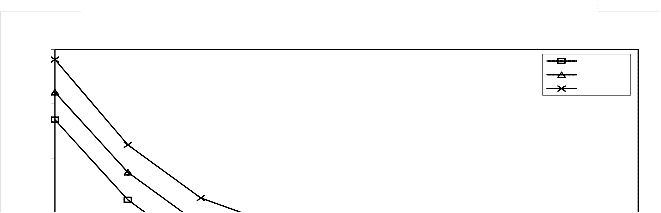
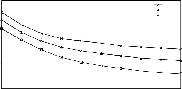
Fig. 3 shows the behaviour of the difference of profits (P1 – P2) with respect to failure rate (α) for different values of the revenue per unit up time (C0). It can be
interpreted from the graph that the difference of profits (P1 –
In steady-state, the number of replacements per unit time is
given by :

P2) decreases with increasing failure rate (α) and has higher values for higher values of the revenue per unit up time (C0). Further, more conclusions can be drawn as follows:

s **(s)

where

lim RP0

RP0 = s0
= D1
(i) For C0 = 55, the difference of profits (P1 – P2) > or = or <
0 if α < or = or > 0.00126. So, the model-I is better or worse than that of model-II according as α < or > 0.00126. In case of
N5 = (p01 + p02) [(1- p34(10)p43(11))(1 – p12(6)p21(7)) -
p14(5) p41(12) (1 - p32(9)p23(8)) + p23(8)(- p32(9) - p41(12)p34(10)p12(6)) + p43(11)(p02 p34(10) - p14(5)p32(9)p21(7)] + p12(6)[(1- p32(9)p23(8)) (p04p41(12) + p01) + p02p21(7) + p41(12) p34(10)(p02 p23(8) + p03) - p34(10) p43(11) p01(1 - p02) + p32(9)p21(7) (p04 p43(11) + p03)] + p21(7)[(1- p14(5) p41(12) ) (p03 p32(9) + p02) + p01p12(6)(1 - p34(10)p43(11)) + p41(12) p12(6)(p34(10) p03 + p04 ) + p32(9)p43(11) (p14(5)p01 + p04 )] + p32(9) [(1- p14(5)p41(12) )(p02p23(8) + p03) - p14(5)p43(11) (p01+ p02p21(7)) – p04p43(11)(1 – p12(6) p21(7)) - p12(6)p21(7) + p12(6)p23(8) (p04 p41(12) + p01)] + p41(12) [(1- p12(6)p21(7)
)(p03 p34(10) + p04 ) + p34(10)p23(8) (p02 + p01p12(6)) +
p01p14(5) (1 – p23(8)p32(9)) + p14(5)p21(7) (p02 + p03 p32(9)
) - p04 p23(8) p32(9)]
and D1 is already specified.

3.10 Profit Analysis

Profit (P2) = C0 (A0) – C2 (BR0) – C3 (BRP0) – C4 (V0) – C5 (RP0)
where
C0 = Revenue per unit uptime.
C2 = Cost per unit uptime for which the expert repairman is
busy for repair.
C3 = Cost per unit uptime for which the expert repairman is
busy for replacement.

C4 = Cost per visit of repairman.
α = 0.00126, both the models are equally good.
(ii) For C0 = 60, the difference of profits (P1 – P2) > or = or <
0 if α < or = or > 0.00135. Therefore, the model of model-I is
better or worse than that of model-II according as α < or >
0.00135 . Both the models are equally good for α = 0.00135. (iii) For C0 = 65, the difference of profits (P1 – P2) > or = or <
0 if α < or = or > 0.00152. So, the model of model-I is better or worse than that of model -II according as α < or > 0.00152. For α = 0.00152, both the models are equally good.
Fig. 4 shows the behaviour of the difference of profits (P1 – P2) with respect to cost per visit for different values of the revenue per unit up time (C0). It can be observed from the graph that the difference of profits (P1 – P2) decreases with increase in the cost per visit and has higher values for higher values of the revenue per unit up time (C0). More conclusions can be drawn as follows:

DIFFERENCE OF PROFIT (P1-P2) vs. FAILURE RATE (α) FOR DIFFERENT VALUES OF THE REVENUE PER UNIT UP TIME (C0)

C 0 = 5 5

C 0 = 6 0

C 0 = 6 5

International Journal of Scientific & Engineering Research, Volume 4, Issue 4, April-2013 408

ISSN 2229-5518

p=0.193, q1=0.706, q2=0.101, =0.000055,

1=0.3206, 2=0.3417, 3=0.1336, C2=1000,

C3=1000, C4=5000, C5 =254838

Failure Rate (α)

Fig. 3

0.15

DIFFERENCE OF PROFIT (P1 - P2) vs. COS T PE R V ISIT FOR DIFFER ENT V ALUES OF THE REV ENU E PER UNIT U P TIM E (C0)

0.1

p=0.193, q1=0.706, q2=0.101, =0.000055,

=0.000015,  =0.3206,  =0.3417,  =0.1336,

C0 = 8

C0 = 9

C0 = 10

1 2 3

0.05

C2=1000, C3=1000, C5 =254838

) 0

2 15000 30000 45000 60000 75000 90000 105000 120000 135000 150000

(P -0.05

-0.1

-0.15

-0.2

COST PER VISIT

Fig. 4
(i) For C0 = 8, the difference of profits (P1 – P2) > or = or < 0 if cost per visit < or = or > INR 28510. So, the model of model-I is better or worse than that of model-II according as cost per visit
< or > INR 28510. In case cost per visit = INR 28510, both the models are equally good.
(ii) For C0 = 9, the difference of profits (P1 – P2) > or = or < 0 if cost per visit < or = or > INR 39750. So, the model of model-I is better or worse than that of model-II according as cost per visit
< or > INR 39750. Both the models are equally good if cost per visit = INR 39750.
(iii) For C0 = 10, the difference of profits (P1 – P2) > or = or < 0 if cost per visit < or = or > INR 60014. So, the model of model-I
is better or worse than that of model-II according as cost per visit < or > INR 60014. If cost per visit = INR 60014, both the models are equally good.

International Journal of Scientific & Engineering Research, Volume 4, Issue 4, April-2013 409

ISSN 2229-5518

Conclusion

After comparison between the two models, we conclude that there are different situations where in a particular model can be preferred over the other model. Depending upon resources available and situations, the organization can adopt the model which is more profitable to it.

References

[1] Attahiru Sule Alfa, W.L. and Zhao, Y.Q., Stochastic analysis of a repairable system with three units and repair facilities. Microelectron. Reliab., 38(4), 585-595 (1998).
[2] Tuteja. R.K., Taneja, G. and Upasana Vashistha, Cost-
benefit analysis of a system where operation and sometimes
repair of main unit depends on sub-unit, Pure and Applied
Mathematika Sciences, LIII(1-2), 41-61(2001).
[3] Gupta, K.C., Sindhu, B.S. and Taneja, G. L., Profit analysis
of a system with patience time and two types of visiting repairman. Journal of Decision and Mathematical Sciences, 7(1-
3), 73-90 (2002).
[4] Tuteja. R.K., Taneja, G. and Parashar B., Probabilistic
Analysis of a PLC Hot Standby System with Three Types of
Failure and Two Types of Repair Facility, Pure and Applied
Mathematika Sciences,Vol. LXIV, No.1-2, Pg. 9 – 20 (2006).
[5] B. Parashar, Statistical Comparative Study of Profit
Analysis of Two Different Models for Two units PLC Systems.
IFRSA’s International Journal of Computing (IIJC), Vol. 1, Issue
2, Pg. 116-128 (2011).