International Journal of Scientific & Engineering Research, Volume 5, Issue 7, July-2014 534

ISSN 2229-5518

2-ELEMENT DIRECTION FINDER FOR OPTIMIZING 2-TIER HETEROGENEOUS NETWORK

D.O Abonyi, P.U. Okafor, M. Alor, Department of Electrical and Electronic Engineering Enugu State University of Science and Technology

Abstract: This paper presents a radio direction finder built with two dipole antennas for use in detecting location of high concentration of mobile phone users for optimum deployment of a pico cell or a femto cell. The design criteria are on low cost and simplicity. Four radiation patterns were generated by selectively altering the phases of the signals arriving at the two antenna elements. W ith a programmed arduino uno board, two 6 bit phase shifters were controlled to electronically alter the phases of the signals arriving at the antennas thereby switching between the beam patterns to monitor the signal strength in form of received signal strength (RSS) of the radio units in front of the array. Directions of arrival (DOA) of the signals were determined by comparing the RSS recorded by each pattern. W ith a two ray propagation model, the locations of the remote radios were estimated with an error margin of 5.30.

Keywords: Radio Direction Finder (RDF), Received Signal Strength Indicator (RSSI), Direction of Arrival (DOA), Phased array antennas, Arduino uno, phase shifters.

1.0 INTRODUCTION

A direction finding system can be described as a device that has the capability of determining the direction of arrival of incident electromagnetic wave. It is able to receive an electromagnetic wave from a distant transmitter, process the signal and determine the signal source direction. Three main steps involved in radio direction finding (RDF) are receiving a signal, characterising the received signal and then processing the data achieved from the characteristics of the received signal. Signals are received with radios designed to receive within the range of frequency for which the signal was transmitted and with its modulation type. The signals are characterised by obtaining some information that describes the received signal like received signal strength (RSS), angle of arrival (AOA), and time of arrival (TOA). One or combination of two or more of these metrics will provide data that will be processed and analysed to determine the actual location or at least an approximated location of the signal source depending on the efficiency of the tool used for the analysis.
Basically, there are three ways by which the direction of arrival of signals can be determined, first by amplitude comparison as used by Khalil in his design of RDF with 8 antenna elements [1], second by phase comparison where beam steering is required [2] and third by time delay comparison. Radio direction finders were known to be complex, large and expensive [3]. Attempts to make it simple and cheap always affect its reliability and performance. Tremendous improvement in localisation systems has been recorded in recent time with the presence of digital technology. Radio direction finder that was initially seen as a big device for the military [4] is now deployed to other areas and currently they are used in radio monitoring, security and surveillance services, military intelligence, communication systems and also in research. With the spread spectrum technique used in wireless communication, the spectral component can only be assigned to a specific emitter if the direction is known. In most direction finders, many antennas are used in an array. It was discovered that sensitivity and element spacing error encountered in old Adcork DF was
reduced with more antenna elements [5] but the more the number of antenna elements, the more complex and costly the system becomes. For this reason, there is need to make a DF as simple and less costly as possible having in mind that accuracy is very important. This paper therefore focused on simulating, building and testing a low cost and still effective DF that can be used to locate mobile phones within a sector of
1200 of a mobile network.

2.0 Basic Antenna array theory

Good result of direction finding is not achieved with a single antenna and so array of antenna is normally used [6, 7]. An antenna array is a combination of two or more antenna element for the purpose of achieving an improved performance. These improved performances can be as an improved gain, diversity reception, interference cancellation in a particular direction, array steering to achieve more sensitivity in a particular direction, determination of DOA of a signal or to maximize the signal to noise ratio of the system. The purpose of using an antenna array is therefore dependent on the aim of exploring one or more of these advantages it can offer over a single antenna. In an antenna array design, a given radiation pattern offered by the array factor is achieved. This factor quantifies the effect of antenna elements in an array without taking into account the individual radiation patterns [8]. The overall radiation pattern of the array is therefore determined by the combination of this array factor and the element radiation factor. Variation in one or more of the following variables affects the overall radiation pattern.
(i) Element arrangement which can be linear, circular,
planar etc.
(ii) Element spacing. (iii) Element excitation
amplitude. (iv) Element excitation phase. (v) Patterns of array element
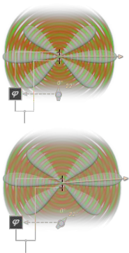
A phased antenna array is composed of radiating elements in an array each connected to a phase shifter. Beams are formed by shifting the phase of the signal received by each radiating element, to provide constructive/destructive interference to steer the beams in the desired direction. Figure 1 [9], show

IJSER © 2014 http://www.ijser.org

International Journal of Scientific & Engineering Research, Volume 5, Issue 7, July-2014 535

ISSN 2229-5518

how the beam of an array can be stirred to a desired direction by varying the phase of the signal received by the different antennas. At 220 phase difference, the main beam was slightly shifted.

Fig 1a two antenna elements, fed with the same phase, (b)

two antenna elements, fed with different phase shift [9].

For an N elements antenna array, assuming X1, X2. . . . .XN are the output of antenna 1 to N and w1, w2. . . . .wN are the weights, then the output of the array is given as;
Where, T is the transpose operator and v(k) is the steering
vector. The array factor, AF is mathematically equal to the
output signal [8].

N

i=1

wi Xi
(1)
For a two element array spaced by half wavelength, assuming a plane wave of constant amplitude is incident on the antennas, the phase of the signal at the antennas will be a function of the angle of arrival of the waves on the antennas. The received signal by antenna i is given by;
The steering vector is a complex vector that represents the relative phase at each antenna. It is dependent on the frequency and propagation direction of the plane wave.

v(k) = e−jkZicosθ°

Xi = e−jkZicosθ

(2)
(5)
Where, θ°is the desired steering angle.
For a desired steering angle of θ° , weights can be applied that
are given by;
Where θ is the angle of arrival of the plane wave, zi is the

2π °

position of each element in the array and k =

λ

is the

wi = ejkZicosθ

magnitude of the wave vector (in radians/meter) which
specifies the phase change per meter for a wave.
(6)
The resulting array factor becomes,
The signals are distinct by a phase factor which is dependent on the antenna separations and the angle of arrival of the
AF = ∑N

ejkZi cosθ ∗ e−jkZicosθ°

(7)
plane wave. Summing the signals of the array, equation 3 is
obtained.
A plot of the array factor against the angle of arrival of the plane wave gives the radiation pattern of the array [9].
S(θ) = ∑N 1

e−jkZicosθ

(3)
Since the array factor is mathematically equal to the output signal, then;
For a phased weighted scheme, the array factor is given by;

S(θ) = ∑N 1 ejkZicosθ ∗ e−jkZicosθ

AF = wT v(k)
(4)
(8)
Where, S(θ) is the output signal from the antenna array.
Considering a progressive phase difference, β between the
antenna elements, equation 8 becomes;

IJSER © 2014 http://www.ijser.org

International Journal of Scientific & Engineering Research, Volume 5, Issue 7, July-2014 536

ISSN 2229-5518

S(θ) = ∑N 1

ej(kZicosθ+β) ∗ e−jkZicosθ°

(9)
and scattering of waves occur as they travel through their paths. In this model, two paths are considered, the line of sight path and the ground reflected path as shown in figure 2.
Equation 9 gives the output signal from antenna array with progressive phase shift between the antennas. For this design, the phase of one antenna is kept at zero while the other is shifted for each instance to produce a radiation pattern with
maximum radiation in the desired direction. Plotting S(θ)
against the angle θ from equation 9 gives the radiation pattern
of the array.

2.5 Received Signal Strength

Two localization algorithms were defined in wireless sensor network, the range based and range free algorithms. In the former, extra hardware is needed to extract the signal strength from the transceiver whereas in the later, no extra hardware is needed. Localization technique based on RSSI measurement is of a range based type. The algorithm uses the inbuilt RSSI circuit in mobile phones [10]. Study have shown that RSSI based algorithm is of low power [11], economical [12] and efficient in a crowded environment with moving human beings [13].
Radios in a network can communicate wirelessly and RSS will be measured by any receiving radio during normal data transfer. The measured RSS can be used to build a localisation algorithm and to estimate the range of the transmitter radio.

3.0 Two ray ground propagation model Transmitted RF energy incurs path loss as electromagnetic waves travel from source to destination. Reflection, diffraction

It is widely used because it has been shown that it gives more accurate path loss estimation at long distances than the free space model [14]. In this case, antenna heights of transmitter and receiver are considered as in equation 10.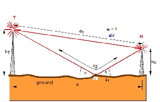

Fig 2: Two ray path loss model

Pr =

PtGtGrht2 hr2

d4

(10)

Table 1: Phase selection

Where; Pr is the receiver power
Pt is the transmitter power
Gt is the transmiting antenna gain
Gr is the receiving antenna gain
ht is the height of transmitting antenna
hr is the height of receiving antenna
d is the distance between Tx and Rx

4.0 Computer Simulation and Results

Simulation was carried out in MATLAB. First simulation of two element radiation pattern based on the above theories to obtain four radiation patterns. Second, 2D plot of randomly scattered nodes was done to represent scattered mobile stations of which their locations are not known. Simulation of RSSI gotten from these nodes and pattern difference was then carried out. Location of one node was then estimated to show an example of how the location of a node can be estimated.

4.1 SIMULATION 1: Two element radiation pattern

A two element radiation pattern was simulated in MATLAB for different phases between the elements using equation 10. Out of the generated patterns and considering what is obtainable with the phase shifters to be used, four phases were selected to cover the required 1200 sector of a normal mobile sectored network. The selected phases in relation to pin configurations of the MAP_010164 phase shifters used for implementation are as shown in table 1.
where D1 - D12 are the feeding points of the arduino uno to
achieve the desired phases β1 for antenna 1 and β2 for
antenna 2.
A polar plot of the four patterns produced by these phase differences and showing their coverage of the required sector from 30 to 150 degrees giving a 120degree coverage is shown

IJSER © 2014 http://www.ijser.org

International Journal of Scientific & Engineering Research, Volume 5, Issue 7, July-2014 537

ISSN 2229-5518

in figure 3.

Radiation pattern of four selected phase groups

120

90 2

60

1.5

150

1 30

0.5

180 0

210

330

240

270

300

Fig 1: Radiation pattern of four selected phase combination for 1200 coverage

Maximum Range Calculation

Considering the sensitivity of XBee-PRO module which is -
102dBm and transmit power of 50mW [15], the maximum
range can be calculated. It was also assumed an isotropic
condition where Gt = Gr = 1. ht and hr were calculated by
measuring the transmit antenna height placed on a desk to the
middle of the antenna and the receive antenna height was determined by measuring to the middle of the antenna when the bracket on which the antenna stands seats on the floor.
ht = 0.46m and hr = 0.52m. These were substituted into
equation 10 to obtain a maximum range of approximately
461meters.
Considering that a base transceiver station in a mobile network is always sectored to 120degrees coverage, this work was then based on 1200 coverage. In this simulation, only values of nodes within the coverage distance and sector are considered.
The broadside pattern array is therefore steered 600 left or right to provide the 1200 required coverage. Nodes formed 61
to 90degrees off broadside in both left and right are not considered in this simulation

4.2 SIMULATION 2: Node Generation

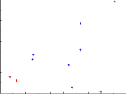
A MATLAB code was written to generate ten randomly scattered nodes representing the mobile users randomly located whose location is to be estimated. It is assumed that the receiver is located at the origin of the x-y coordinates of the plot. The distance of these nodes from the origin was then calculated by the code using Pythagoras theory. If the distance of each node is less than the maximum distance which was calculated from a two ray path loss model of equation 12 to be
461meters, the receiver is meant to receive the signal from that
node otherwise, the node is indicated as ‘’out of range’’. On
the other hand if the angle, θ is less than 60degree both left
and right, it indicates it is ‘’out of range’’ too, where θ is the angle off broadside. A sample plot of randomly generated scatter nodes is shown in figure 4 where the nodes marked with red are those that are out of range which the system does not care about.

450

400

350

300

250

200

150

100

50

0

Plot1

Pythagoras equation. Y axis ranges from 0 to 461 while x axis is also a 461m range with zero located in the middle. A right angled triangle is formed from the coordinator to each of the nodes giving the straight line distance with the already known x and y values of each node.

RSSI measurement

A two ray path loss model equation was incorporated in the code to determine the received signal strength in the form of RSSI in dBm received from the nodes. Table 2 shows the data recorded by this program for an instance of a randomly scattered plot (plot1 above). Theta is the angle off broadside. Values marked with ‘**’ are those reported to be ‘out of range’.

-250 -200 -150 -100 -50 0 50 100 150 200 250

x axis

Fig 2: Randomly scattered Nodes

Line of sight distance measurement
The code also measures a strength line distance, d(i) of each node to the coordinator located at the origin using the

Table 2: Simulation result sample

IJSER © 2014 http://www.ijser.org

International Journal of Scientific & Engineering Research, Volume 5, Issue 7, July-2014 538

ISSN 2229-5518

where Gt = Gr = 1 and also for antenna gains. For each of the scattered nodes with a LOS distance, a received power Pr(i) is calculated by the code using the two ray path loss model in dBm to give the received signal strength for each node (RSSI(dBm)). Results generated are shown in table 4

4.3 SIMULATION 3: RSSI Verses Pattern difference

Here the RSSI from ten scattered nodes are considered in relation to the different radiation patterns for isotropic case Table 3: Angle of maximum radiation of each pattern
Matlab code was used to plot a non-normalised radiation pattern for the four beam patterns considered in this study. Each of the beam patterns produces a highest gain at different angles depending on the direction of the main lobe of the beam. It was observed that the highest gain for all pattern was
3.01dB and that this value is achieved by the different patterns at the following angles as shown on table 3;
This justifies the fact that these patterns will receive signals arriving within the region of these angles with more signal strength than any other pattern. Some angles on the broadside and to the left and right off the broadside were selected as shown on the table to carry out this simulation. 10 nodes representing scattered mobile users are involved. A negative x indicates that the node is to the left of the broadside and positive x indicates that the node is on the right of broadside. Since a broadside pattern is used as reference, 900 on the pattern represents a 00 on the graph and angle to the right is angle off broadside subtracted from 900 while angle to the left is the angle off broadside added to 900. This keeps both the
nodes and the pattern at the same angle off broadside for clearer analysis. Results obtained from randomly scattered nodes in relation to the four patterns are shown in table 5.
From table 4, it can be deduced that patterns will receive highest RSSI value at the following regions because that is their region of highest gain when compared with other patterns. From antenna theory, the higher the gain, the better the reception or transmission. Analysis will be based on this as expectation is on receiving a better signal with higher RSSI at angles of maximum gain for each pattern.

Table 4: Region of highest radiation by different patterns

4.4 Simulation Results

Data obtained from the scattered nodes RSSI measurement and the simulation of the two element array are tabulated as

Table 5: Simulation result for Isotropic nodes

in tables 6,7 and 8 for analysis. Negative x indicates that the node is located on the left. It is assumed that x and d are not known.

IJSER © 2014 http://www.ijser.org

International Journal of Scientific & Engineering Research, Volume 5, Issue 7, July-2014 539

ISSN 2229-5518

Table 6: Simulation result for non-isotropic nodes

Result Analysis

From tables 5 and 6 above, it can be seen that;
• The higher the distance for the same angle, the smaller the measured RSSI as seen in nodes8 and 9.
• Node 3 occurred at the same LOS distance and in same direction for both isotropic and antenna gain considerations. The difference in their RSSI value gives 7.2dB. This means that this antenna array has a
7.2dB gain above isotropic.
• It can be deduced that a pattern with highest RSSI value, a value closer to zero has the most likelihood of having the node at its region. For instance, node 1 is most likely to be located within the region of PI left or right while node 6 will most likely be located within the region of P2.
• It can also be noticed that patterns P2 and P3 are symmetrical, while one has maximum reception in one direction, the other one has maximum in the opposite direction.
• Pattern 4 gives the same gain for the same angle in both left and right as seen in node 6 and 7.
Considering that the array has a gain of 7.2dBi from simulation result as indicated above, another table showing the array gain over isotropic as shown in table 8 is developed;

5.0 Direction Finder test

The DF was physically tested in the mappin hall of The University of Sheffield with 7 nodes and one coordinator. There is no defined command for arduino-XBee pro serial 2 as it is in serial 1, ‘’getRssi()’’ for extracting out RSSI value from a received packet [16]. The inability for the command ‘’get RSSI’’ to work with arduino/XBee pro s2 made the final testing to be switched over to using waspmote setup.

5.1 Set up for testing

An XBee Pro s2 (with a small dipole antenna) module configured as a router in API mode and connected to a waspmote board which was powered with a 5V battery and programmed in C++ were used as the nodes. The coordinator
was a waspmote board and Xbee Pro s2 powered with 5V battery and connected to a personal laptop to display the received packets which include the RSSI values. The two element array were used as the coordinator antenna and the phase between the antennas were manually shifted by supplying a high or a low to the data pins of the phase shifters as required using a digital power supply. RSSI values were reported and extracted from the packets received from the nodes and then recorded with a personal computer. Table 1 indicates the average value of 6 measurements from each of the nodes. Using Cisco look up conversion table for RSSI to dBm values as shown in Appendix A, the measured RSSI values were converted to dBm to show the received signal strength for the different phase values which produce the different patterns indicated as P1-P4. Figure 5 show the set up at mappin hall for the DF testing.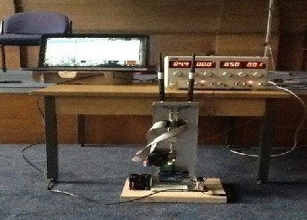

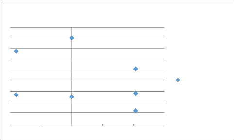
Fig 5: Coordinator set up

5.2 Node distribution for test

The nodes were distributed within the mapping hall of The University of Sheffield, UK as shown in table 7 and plotted in figure 6. Nodes were configured with personal Identity number to avoid ambiguity in the network received data. The Range describes the measured distance from the coordinator located in the origin of the plot. This distance is not known but

IJSER © 2014 http://www.ijser.org

International Journal of Scientific & Engineering Research, Volume 5, Issue 7, July-2014 540

ISSN 2229-5518

was measured to test the result for Range calculation of the direction finder

Table 7: Node distribution for DF test

NODES
NODES ID
RANGE, d(m)

Node distribution

18

16

14

12

10

8

6

4

2

0

Node distribution

-4 -2 0 2 4 6

Fig 6: 2D graph of node distribution for testing DF

Communication between Radios

In other to get the signal strength from the radios, they need to communicate and send packets to each other so as to measure
acknowledgement to be received. On receiving ACK from the last see the network, it then sends scfRSSI message to each of the nodes and wa node to scan for available brother nodes around. The node then sen
the strength of the signal received from them. For radios to communicate they must have the same PAN ID and for this reason, all radios in this work are set to PAN ID
0102030405060708. Waspmote board were programmed to
control the sending and receiving of packets through the XBee
modules. One coordinator and 7 routers are involved all configured in API mode.
message to each of the brothers who by responding allows him to meas
RSSI and report back to the coordinator who then measures the RSSI
him and the node. Table 8 Show the measured RSSI values from the n their values in dBm as looked up from the Cisco RSSI/dBm conversion

Table 8: Measured Data

Programming Routers

The routers are programmed in C++ to be in a waiting mode waiting for a message from the coordinator. They respond to a packet received, from the coordinator who sends a test message to them in turns. They find out brother nodes in the same network around them and report back to the coordinator introducing himself, his ID, MAC address, RSSI value between him and the coordinator as well as other brother nodes around him with the signal strength between himself and those brothers. For the purpose of this research where we need to find how the signal from each of these nodes are received by the different beam patterns produced by phase shifting the signals arriving at the antennas, only the RSSI data between each of the scattered nodes and the coordinator will be used in our analysis.

Programming the coordinator

5.3 Result Analysis

The coordinator is programmed in C++ to scan the network and fine thTeheradrieocseived signal strength is inversely related to the
in his network and note how many they are. It then sends a test messadgiesttaontcheeas expressed in path loss equation. The farther the
routers one at a time and wait for a maximum of three minutes for an

IJSER © 2014 http://www.ijser.org

International Journal of Scientific & Engineering Research, Volume 5, Issue 7, July-2014 541

ISSN 2229-5518

distance between two radios, the smaller the signal strength. As discussed earlier, the pattern receiving a particular node at the highest signal strength is the pattern that has the node in its region. Knowing the angle region of maximum reception of each pattern, the location of each node can be estimated to an acceptable accuracy. The following points can be drawn from the measured data;
The pattern with highest RSSI (dBm) reading indicates the region of location of the node.
Nodes 2, 4 and 7 are located at the region of P1, 1 and 5 at the region of P2, node 3 at the region of P3 and nodes 6 at the region of P4.
Second highest RSSI value pattern is also a necessary factor to determining the location of the nodes, left or right of the broadside.
P2 being the second highest RSSI reading for node 2 after P1 indicates that node 2 is right of broadside and not left.
The second highest pattern also helps to narrow down the localisation of the node to a better accuracy as demonstrated in simulation and to be shown again in next subsection.
A better RSSI value is achieved at far field because the radiation pattern is designed under far field condition as can be seen in the reception and RSSI measuring of nodes 2 and 7 where 7 is place 16meters from the coordinator and node 2 just 5meters away but node 7 showed a stronger signal than node 2.

Localisation

From the received RSSI values, P2 has the highest received RSSI value therefore Node 1 is within the range of Pattern 2 (P2) which is 19-540off broadside, right. The second highest is node 1 which has its value between 0 and 180 right. Halving the coverage area of P2 in favour of P1 to give 17.50 as done in simulation and finding the percentage difference between them to give 3.5%. This percentage of 3.5% will give approximately 1.2 which can be subtracted from the minimum range value added to half the range value to give a location estimate of 19+17.50-1.2 = 35.30 with an error margin of 5.30.

6.0 CONCLUSION

A two dipole element direction finder has been discussed. By altering the phase of the signal received by each antenna, different beam patterns are formed. Switching between four different patterns of the array, signals in front of the arrays are received and their RSSI measured. Using a two ray propagation model, the distance of the signal source from the receiver is obtained and the location of the source is determined by comparing the received signal strength from each of the patterns. The pattern with highest RSSI value has the node in its region (pre-determined) and the location can be further narrowed down by relating the pattern with next highest RSSI value to the highest RSSI value pattern. Location is achieved with acceptable error margin. The design objective is achieved by its simplicity and low cost.

REFERENCES

[1] K. Ibrahim, and D. Mohammad, "Design of Wideband Radio Direction Finder Based On Amplitude Comparison," Al-Rafidain Engineering, vol. 19 No.5, pp. 77-86, Oct. 2011.
[2] W. Diab, and H. Elkamchouchi, "A Deterministic
Real-Time DOA-Based Smart Antenna Processor,"
The 18th Annual International Symposium On
Personal, Indoor, and Mobile Radio
Communications (PIMRC 07), 2007.
[3] M. Stieber, "Radio Direction Finding Network
Receiver Design for Low-Cost Public Servive
Application," MEng. Thesis, California Polytechnic
State University, Dec. 2012.
[4] K. Williams, "Secret Weapon – U.S. High – Frequency Direction Finding in the Battle of the Atlantic, Annapolis," Naval lnstitute Press, 1996.
[5] D. Travers, "Spacing-error analysis of the eight- element two-phase adcork direction finder,"
Antennas and Propagation, IRE Transactions on, vol.3, no.2, pp. 63,65, April 1955.
[6] C. Plapous, C. Jun, E. Taillefer, A. Hirata, and T.
Ohira, "Reactance domain MUSIC algorithm for
electronically steerable parasitic array radiator,"
Antennas and Propagation, IEEE Transactions on, vol. 52, pp. 3257-3264, 2004.
[7] A. Hirata, E. Taillefer, H. Yamada, and T. Ohira, "Handheld direction of arrival finder with electronically steerable parasitic array radiator using the reactancedomain MUltiple SIgnal Classification algorithm," Microwaves, Antennas & Propagation, IET, vol. 1, pp. 815-821, 2007.
[8] G. Moernaut and D Orban, "The Basics of Antenna
array," Orban Microwave Products,Available: www.orbanmicrowave.com. Last accessed on 28th March 2014.
[9] Antennas, Available online at:
http://www.radartutorial.eu/06.antennas/an14.en.html.
last accessed on 7th April 2014
[10] D.-x. Fu, D.-q. Feng, and H.-n. Zhang, "Mean LQI
and RSSI based link evaluation algorithm and the
application in frequency hopping mechanism in
wireless sensor networks," in Consumer Electronics,
Communications and Networks (CECNet), 2011
International Conference on, 2011, pp. 3252-3257.
[11] R. Jin, H. Wang, B. Peng, and N. Ge, "Research on
RSSI-Based Localization in Wireless Sensor
Networks," in Wireless Communications,
Networking and Mobile Computing, 2008. WiCOM
'08. 4th International Conference on, 2008, pp. 1-4.
[12] R. Al Alawi, "RSSI based location estimation in
wireless sensors networks," in Networks (ICON),
2011 17th IEEE International Conference on, 2011,
pp. 118-122.

IJSER © 2014 http://www.ijser.org

International Journal of Scientific & Engineering Research, Volume 5, Issue 7, July-2014

ISSN 2229-5518

[13] S. Hara and D. Anzai, "Experirrental Performance [15] Comparison of R:>SI- and TDOA-Based IDeation

Estimation Methods," in Vehicular Technology

Conference, 2008. VTC Spring 2008. IEEE, 2008, pp. [16]

2651-2655.

[14] J. Andrusenko, "Modeling and Simulation for RF

Propagation/The John Hopkins University, applied physics lab, Dec. 2009.

IJSER © 2014

http /fwww ijser org

542

XBee data sheet by Digi international Inc. Available online at: http:/ /www.digi.com Last accessed on

9th April 2014

Value reading, Available online at:

http:/ /www.digi.com/support/forum/6135/ rssi value-Reading. Last accessed on 17th April2014.